Registered S3 method overwritten by 'quantmod':
  method            from
  as.zoo.data.frame zoo
Loading required package: carDataUnderstanding the statistical properties of financial data is fundamental to effective risk management and investment decision-making. Financial returns exhibit characteristics that often deviate significantly from the assumptions underlying classical statistical theory, particularly the assumption of normality that underpins many traditional models.
This chapter explores the descriptive statistics most relevant to financial analysis, focusing on measures that capture the unique properties of return distributions. We examine basic summary statistics such as mean and volatility, but also delve into normalised moments like skewness and kurtosis that reveal asymmetries and tail behaviour often overlooked in standard analysis.
The chapter demonstrates how to test distributional assumptions using formal hypothesis tests, visualise return distributions through various plotting techniques, and compare the statistical properties across different assets. We also explore autocorrelation patterns that reveal important features like volatility clustering in financial time series.
R is particularly well-suited for this type of statistical analysis. It has considerable depth in various statistical procedures built in, along with specialised statistical packages for advanced techniques one cannot find elsewhere. The language’s extensive library of statistical tests, distribution functions, and visualisation tools makes it an ideal platform for the comprehensive analysis of financial data properties.
Throughout, we use real financial data to illustrate these concepts, showing how the statistical properties of returns have practical implications for portfolio construction, risk assessment, and model validation. The tools and techniques covered here form the foundation for more advanced econometric and risk modelling approaches discussed in later chapters.
Registered S3 method overwritten by 'quantmod':
method from
as.zoo.data.frame zoo Loading required package: carDatalibrary(moments)
library(ggplot2)
library(tseries)
library(car)
library(lubridate)
library(zoo)
library(reshape2)
source("common/functions.r",chdir=TRUE)data=ProcessRawData()
Price=data$Price
Return=data$Return
sp500=data$sp500The first step in analysing financial return distributions is calculating basic descriptive statistics that summarise key characteristics of the data. These statistics provide useful insights into the central tendency, dispersion, and distributional shape of returns - all important factors for risk assessment and portfolio management.
The following statistics form the foundation of financial analysis: mean return indicates expected performance, standard deviation measures volatility or risk, whilst skewness and kurtosis reveal departures from normality that have implications for risk management and option pricing models.
We begin with the four fundamental statistics. Mean and standard deviation are directly built into R, while skewness and kurtosis require the library(moments) package:
mean(sp500$y)[1] 0.0003186239sd(sp500$y)[1] 0.01143725skewness(sp500$y)[1] -0.3620415kurtosis(sp500$y)[1] 13.81192With more formatted printing.
cat('Sample statistics for the S&P 500 from',
 min(sp500$date),'to',
 max(sp500$date),'\n'
)
Sample statistics for the S&P 500 from 19900103 to 20250630 We can present these results a bit nicer by putting them into a data frame.
stats = c('mean:', paste0(round(mean(sp500$y)*100,3),'%'))
stats = rbind(stats, c('sd:', paste0(round(sd(sp500$y)*100,2),'%')))
stats = rbind(stats, c('skewness:', round(skewness(sp500$y),1)))
stats = rbind(stats, c('kurtosis:', round(kurtosis(sp500$y),1)))
stats = as.data.frame(stats)
names(stats) = c("Name","Value")
rownames(stats) = NULL
print(stats)
Name Value
1 mean: 0.032%
2 sd: 1.14%
3 skewness: -0.4
4 kurtosis: 13.8Or printing them with formatting.
for(i in 1:dim(stats)[1])
 cat(stats[i,1],rep("",10-nchar(stats[i,1])),stats[i,2],"\n")
mean: 0.032%
sd: 1.14%
skewness: -0.4
kurtosis: 13.8 For portfolio analysis, it is often useful to compare statistical properties across multiple assets simultaneously. We can create a comprehensive summary table for all stocks in our dataset:
# Calculate statistics for all stocks
stats_summary = data.frame(
  Asset = names(Return)[2:ncol(Return)], # Exclude date column
  Mean = sapply(Return[,2:ncol(Return)], function(x) round(mean(x, na.rm=TRUE)*100, 3)),
  SD = sapply(Return[,2:ncol(Return)], function(x) round(sd(x, na.rm=TRUE)*100, 2)),
  Skewness = sapply(Return[,2:ncol(Return)], function(x) round(skewness(x, na.rm=TRUE), 2)),
  Kurtosis = sapply(Return[,2:ncol(Return)], function(x) round(kurtosis(x, na.rm=TRUE), 2))
)
print(stats_summary, row.names = FALSE)
Asset Mean SD Skewness Kurtosis
AAPL 0.126 2.12 -0.10 8.34
DIS 0.037 1.76 0.22 12.57
GE -0.006 2.04 -0.07 12.06
INTC 0.019 1.98 -0.45 11.97
JPM 0.044 2.28 0.27 20.64
MCD 0.066 1.33 0.11 19.04This comparative view reveals important differences across assets. Technology stocks like AAPL and NVDA typically show higher volatility, whilst financial stocks like JPM may exhibit different skewness patterns. Assets with kurtosis values significantly above 3 indicate heavier tails than the normal distribution, suggesting higher probability of extreme returns.
The systematic comparison helps identify which assets contribute most to portfolio risk and which exhibit the most pronounced departures from normality assumptions commonly used in traditional finance models.
R provides functions for just about every distribution imaginable. We will use several of those: the normal, student-t, skewed student-t, chi-square, binomial and the Bernoulli. They all provide densities and distribution functions (PDF and CDF), as well as the inverse CDF and random numbers discussed in Chapter 13.
The first letter of the function name indicates which of these four types, d for density, p for probability, q for quantile and r for random. The remainder of the name is the distribution, for example, for the normal and student-t:
dnorm, pnorm, qnorm, rnorm;dt, pt, qt, rt.dnorm(1)[1] 0.2419707pnorm(1.164)[1] 0.877788qnorm(0.95)[1] 1.644854If you want to plot the distribution functions, first create a vector for the x coordinates with seq(a,b,c) which creates a sequence from a to b where the space between the numbers is c. Alternatively, we can specify the number of elements in the sequence.
x = seq(-3,3,length=100)
z = seq(0,1,length=100)
plot(x,dnorm(x), main="Normal density",type='l')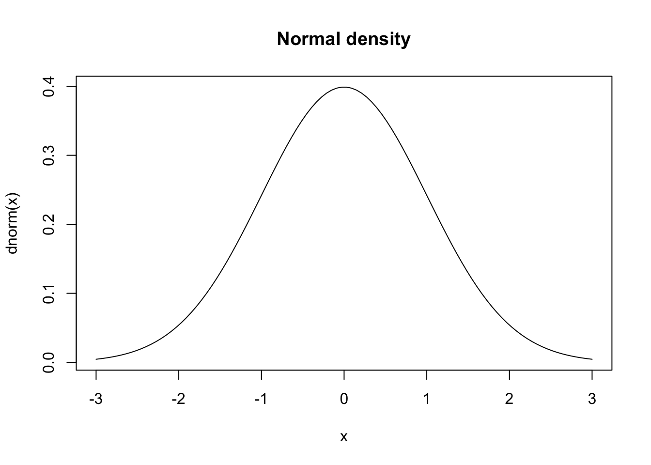
plot(x,pnorm(x), main="Normal distribution",type='l')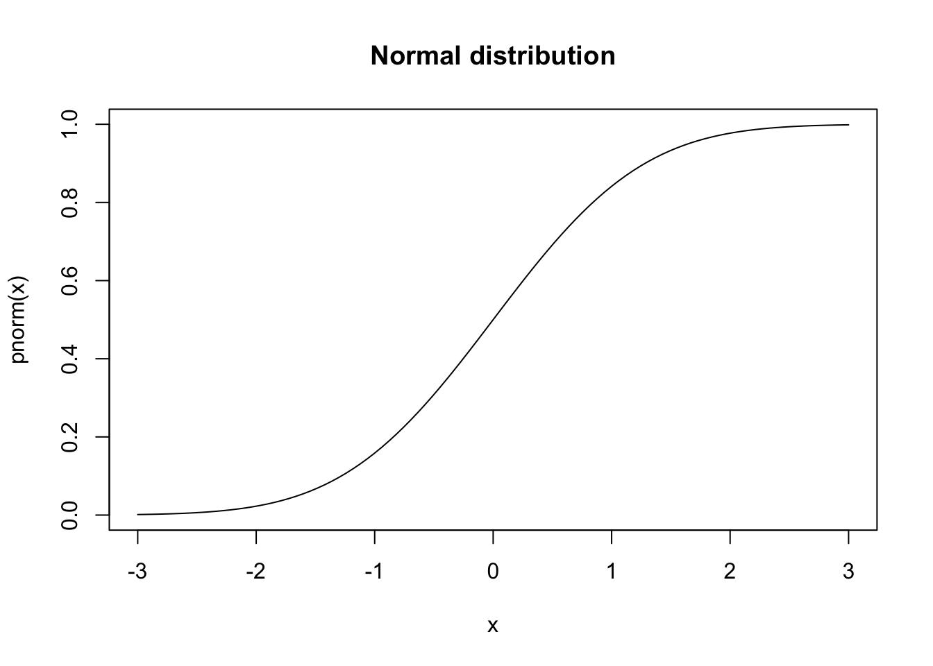
plot(z,qnorm(z), main="Normal quantile",type='l')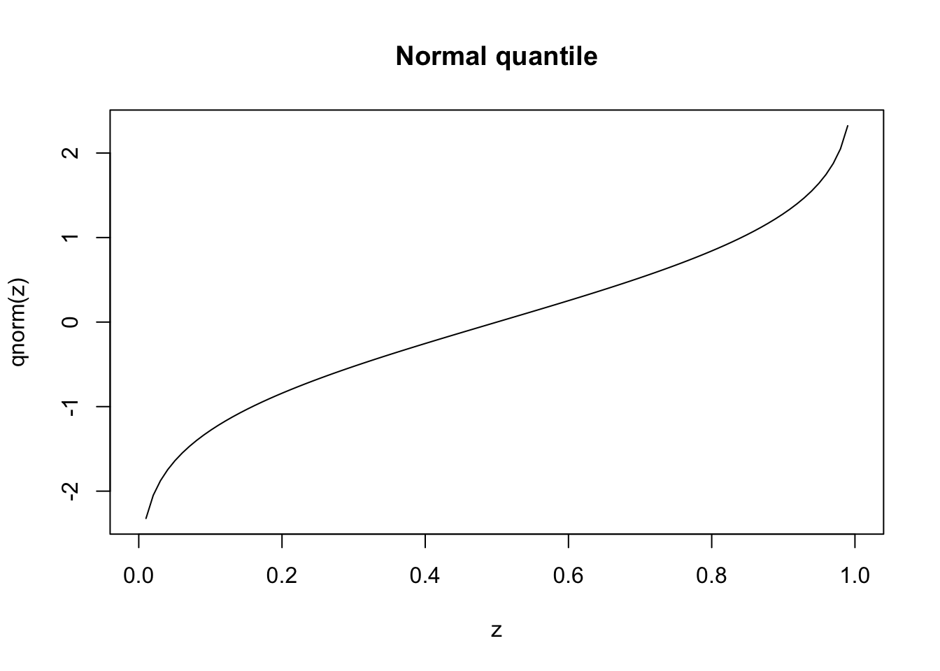
These visualisations provide intuitive understanding of distributional properties, but formal statistical tests are needed to make objective assessments about the data’s characteristics.
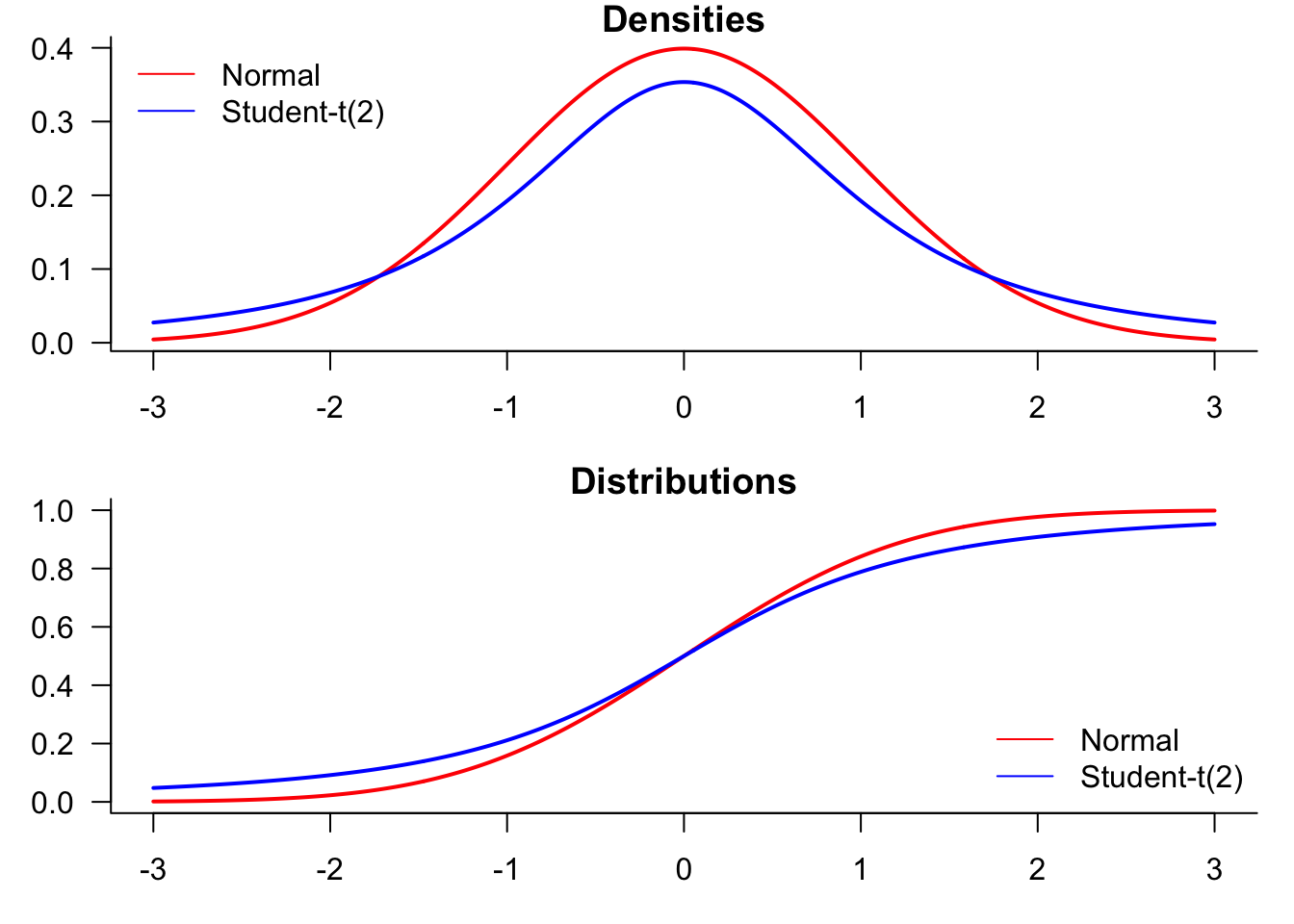
We start by generating a plot comparing normal and t-distributions. T-distributions are heavy-tailed and convenient when we need fat-tailed distributions. The following plot highlights the difference between normal and t-distributions.
x=seq(-3,3,length=500)par(mfrow=c(2,2),mar=c(3,3,1,1))
plot(x,dnorm(x),type="l", lty=1, lwd=2, main="Normal PDF",
xlab="x", ylab="Probability") # normal density
plot(x,dt(x,df=2),type="l", lty=1, lwd=2, main="Student-t(2) PDF",
xlab="x", ylab="Probability") # t density
plot(x,pnorm(x),type="l", lty=1, lwd=2, main="Normal cdf",
xlab="x", ylab="Probability") # normal cdf
plot(x,pt(x,df=2),type="l", lty=1, lwd=2, main="Student-t(2) cdf",
xlab="x", ylab="Probability") # t cdf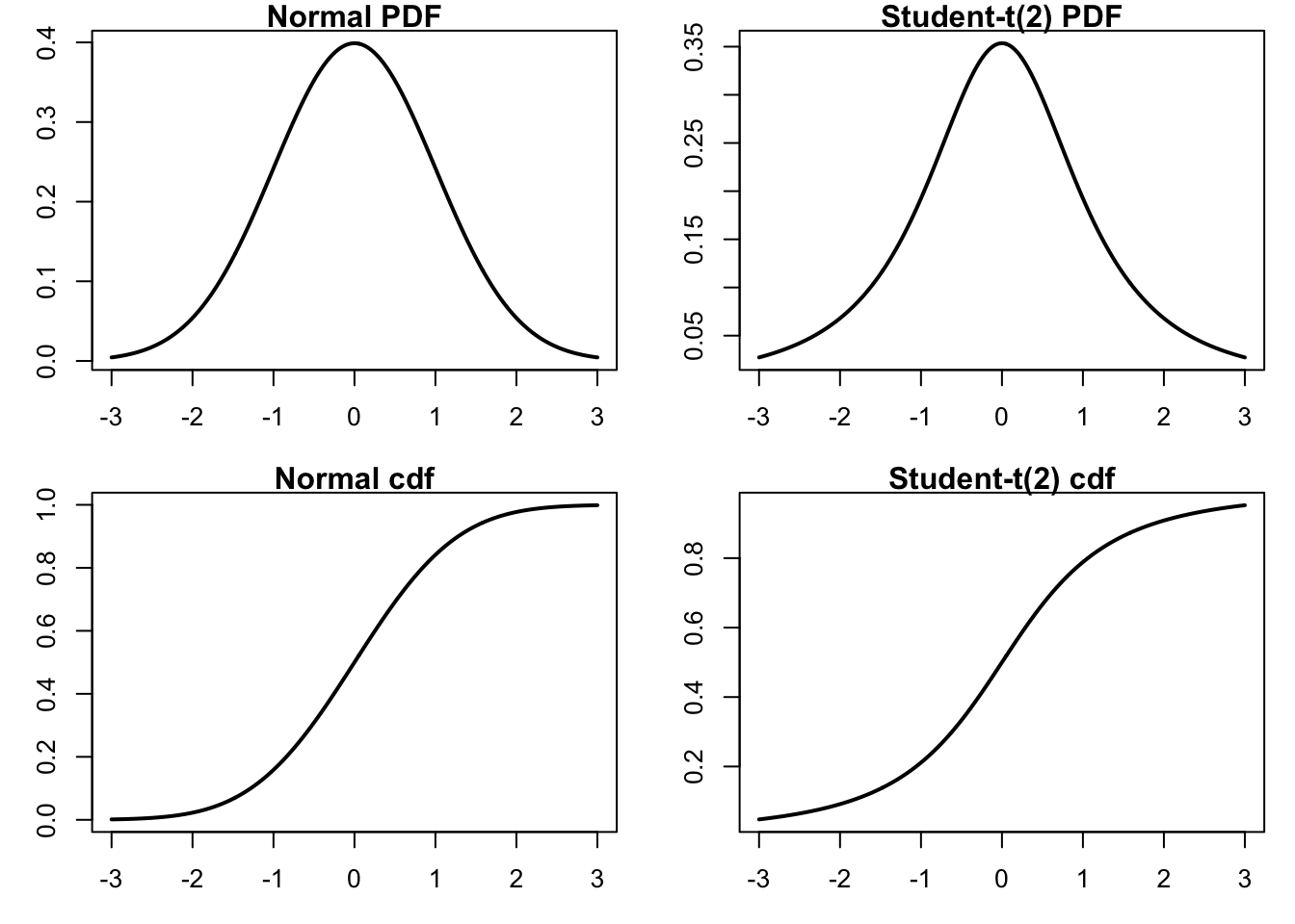
To compare the distributions, it might be better to plot them both in the same figure.
par(mfrow=c(2,1),mar=c(3,3,1,1))
plot(x,dnorm(x),
     type="l",
     lty=1,
     lwd=2,
     main="Densities",
     xlab="value",
     ylab="Probability",
     col="red",
     las=1,
     bty='l'
)
lines(x,dt(x,df=2),
     type="l",
     lty=1, lwd=2,
     col="blue"
)
legend("topleft",
     legend=c("Normal","Student-t(2)"),
     col=c("red","blue"),
     lty=1,
     bty='n'
)
plot(x,pnorm(x),
     type="l",
     lty=1,
     lwd=2,
     main="Distributions",
     xlab="x",
     ylab="Probability",
     col="red",
     las=1,
     bty='l'
)
lines(x,pt(x,df=2),
     lwd=2,
     col="blue"
)
legend(
     "bottomright",
     legend=c("Normal","Student-t(2)"),
     col=c("red","blue"),
     lty=1,
     bty='n'
)
Statistical hypothesis testing provides formal methods for evaluating distributional assumptions and properties of financial data. These tests help determine whether observed patterns are statistically significant or could reasonably be attributed to random variation.
The tests covered in this section address common questions in financial analysis: Are returns normally distributed? Do they exhibit serial correlation? How well do they fit theoretical distributions? Each test provides a p-value that indicates the probability of observing the data under the null hypothesis, allowing for objective assessment of distributional assumptions.
The Jarque-Bera (JB) test in the tseries library uses the third and fourth central moments of the sample data to check whether its skewness and kurtosis match a normal distribution.
jarque.bera.test(sp500$y)
    Jarque Bera Test

data:  sp500$y
X-squared = 43730, df = 2, p-value < 2.2e-16
The p-value presented is the inverse of the JB statistic under the CDF of the asymptotic distribution. The p-value of this test is virtually zero, which means that we have enough evidence to reject the null hypothesis that our data has been drawn from a normal distribution.
This result has important practical implications: risk models that assume normally distributed returns will systematically underestimate the probability of extreme market movements. The rejection of normality suggests that alternative distributions (such as student-t) may be more appropriate for risk management applications.
The Kolmogorov-Smirnov test, ks.test() is based on comparing actual observations with some hypothesised distribution, like the normal:
x = rnorm(n=length(sp500$y))
z = rnorm(n=length(sp500$y))
ks.test(x,z)
    Asymptotic two-sample Kolmogorov-Smirnov test

data:  x and z
D = 0.020139, p-value = 0.0533
alternative hypothesis: two-sided
This confirms we fail to reject the null hypothesis.
x = rnorm(n=length(sp500$y))
ks.test(x,sp500$y)
Warning in ks.test.default(x, sp500$y): p-value will be approximate in the
presence of ties
    Asymptotic two-sample Kolmogorov-Smirnov test

data:  x and sp500$y
D = 0.48646, p-value < 2.2e-16
alternative hypothesis: two-sided
x = rt(df=3,n=length(sp500$y))
ks.test(x,sp500$y)Warning in ks.test.default(x, sp500$y): p-value will be approximate in the
presence of ties
    Asymptotic two-sample Kolmogorov-Smirnov test

data:  x and sp500$y
D = 0.48702, p-value < 2.2e-16
alternative hypothesis: two-sided
The first test comparing S&P 500 returns to normal random numbers shows a very low p-value, confirming non-normality. The second test comparing to t-distributed random numbers with 3 degrees of freedom shows a higher p-value, suggesting that heavy-tailed distributions provide a better fit to financial return data.
The Ljung-Box (LB) test checks if the presented data exhibits serial correlation. We can implement the test using the Box.test() function and specifying type = "Ljung-Box":
x = rnorm(n=length(sp500$y))
Box.test(x, type = "Ljung-Box")
    Box-Ljung test

data:  x
X-squared = 0.52188, df = 1, p-value = 0.47Box.test(sp500$y, type = "Ljung-Box")
    Box-Ljung test

data:  sp500$y
X-squared = 56.298, df = 1, p-value = 6.228e-14Box.test(sp500$y^2, type = "Ljung-Box")
    Box-Ljung test

data:  sp500$y^2
X-squared = 862.14, df = 1, p-value < 2.2e-16
The first test on random normal data shows no significant autocorrelation, as expected. The test on S&P 500 returns shows minimal serial correlation in returns themselves. However, the test on squared returns reveals significant autocorrelation, indicating volatility clustering - periods of high volatility tend to be followed by high volatility periods. This is a key stylised fact of financial markets with important implications for volatility modelling.
The autocorrelation function shows us the linear correlation between a value in our time series and its different lags. The acf function plots the autocorrelation of an ordered vector. The horizontal lines are confidence intervals, meaning that if a value is outside of the interval, it is considered significantly different from zero.
par(mar=c(4,4,3,0))
acf(sp500$y, main = "Autocorrelation of returns")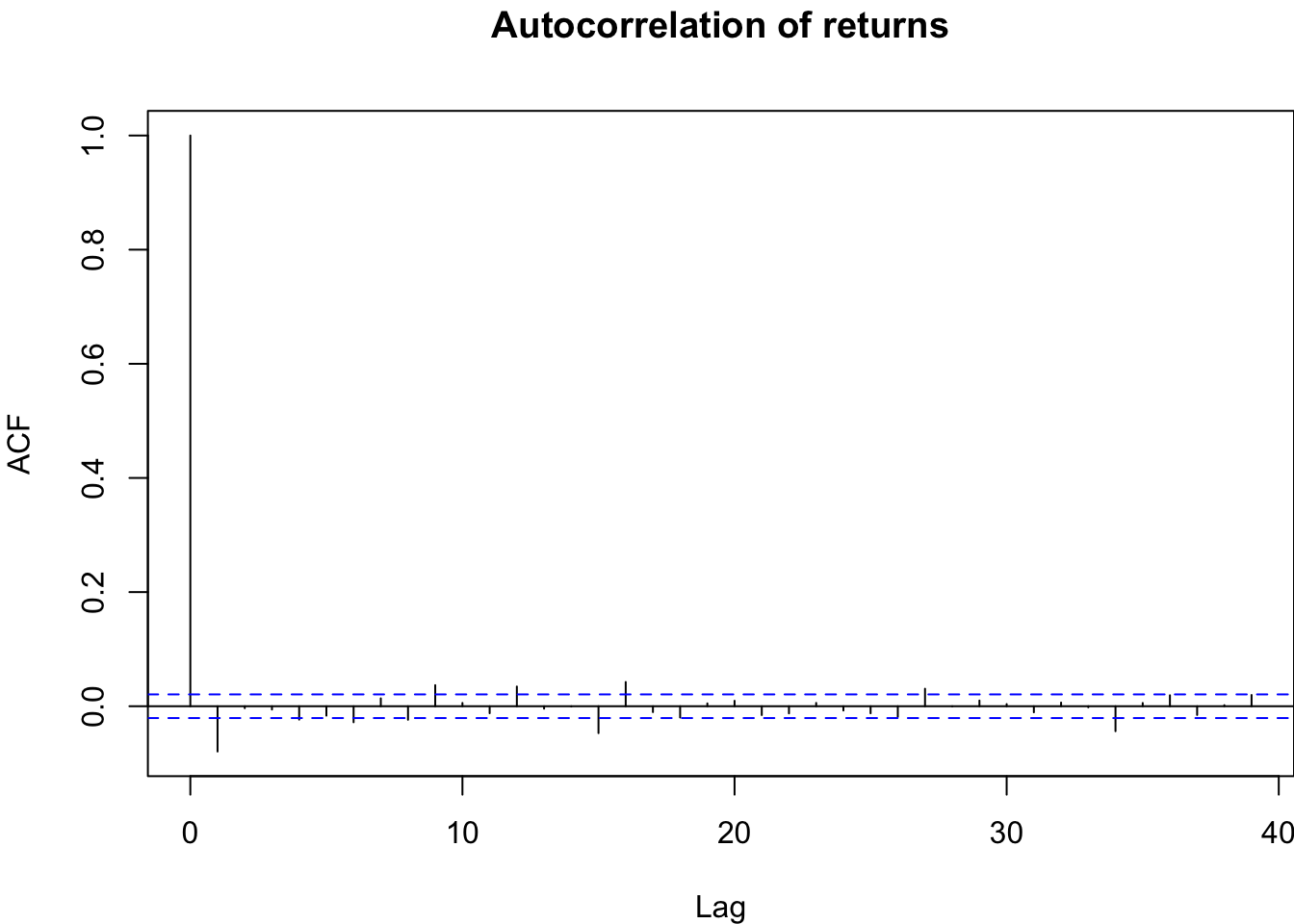
The plots made by the acf function do not look all that nice. While there are other versions available for R, including one for ggplot, for now, we will simply modify the built-in acf(). Call that myACF() and put it into functions.r.
myACF=function (x, n = 50, lwd = 2, col1 = co2[2], col2 = co2[1], main = NULL)
{
 a = acf(x, n, plot = FALSE)
 significance_level = qnorm((1 + 0.95)/2)/sqrt(sum(!is.na(x)))
 barplot(a$acf[2:n, , 1], las = 1, col = col1, border = FALSE,
 xlab = "lag", ylab = "ACF", main = main)
 abline(significance_level, 0, col = col2, lwd = lwd)
 abline(-significance_level, 0, col = col2, lwd = lwd)
 axis(side = 1)
}
par(mar=c(4,4,1,0))
myACF(sp500$y, main = "Autocorrelation of S&P 500 returns")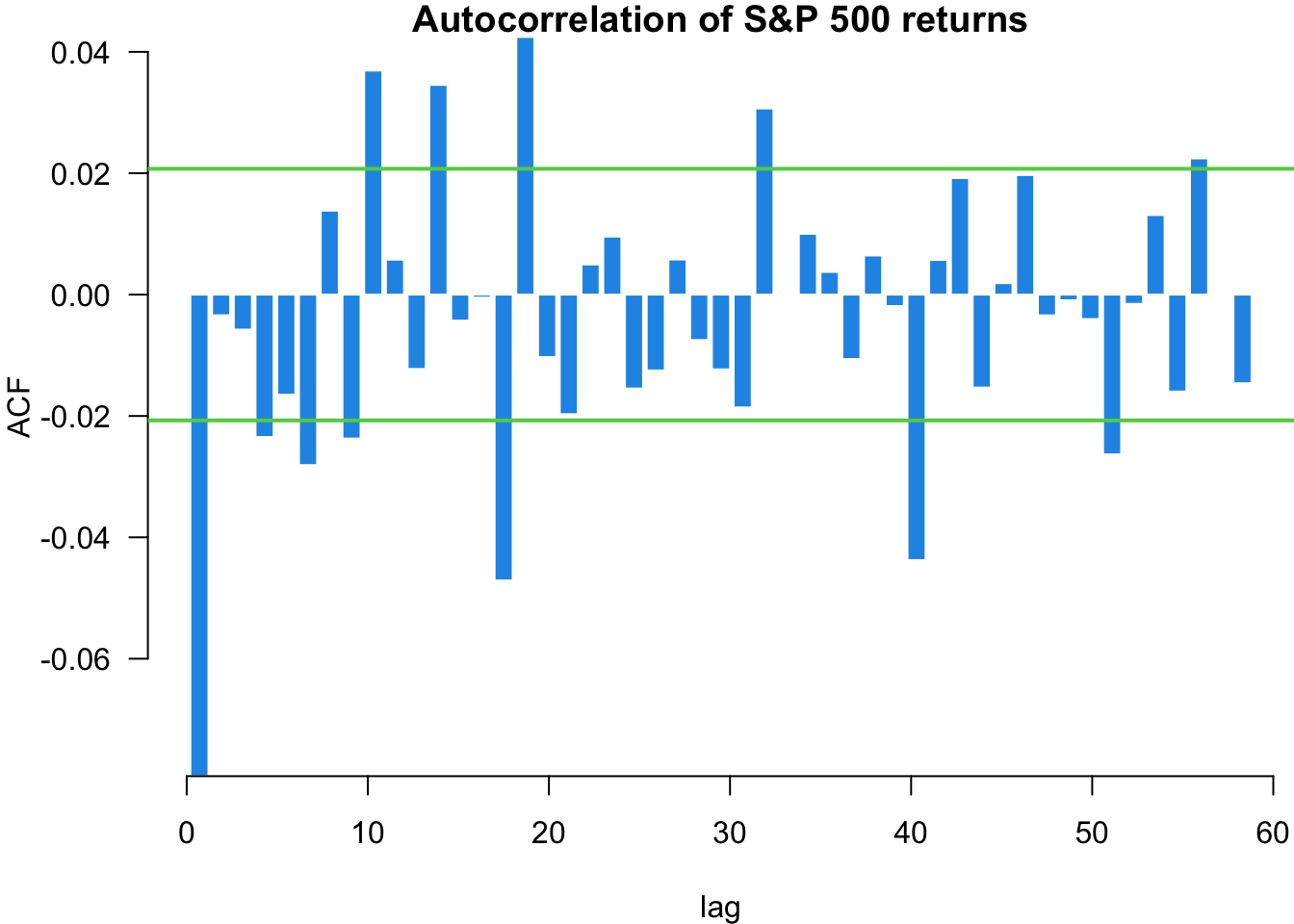
myACF(sp500$y^2, main = "Autocorrelation of squared S&P 500 returns")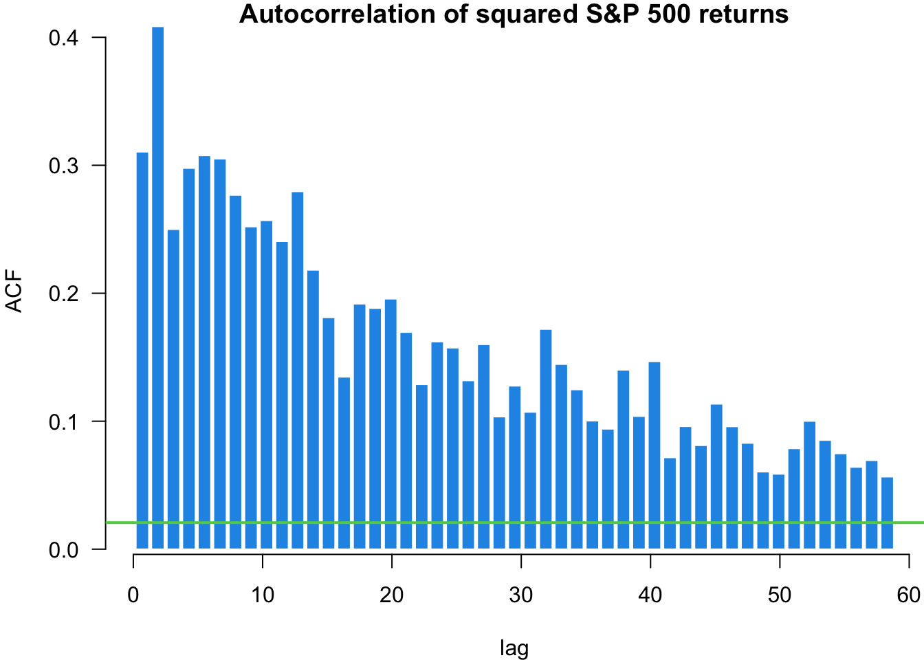
We can use the quantile-quantile (QQ) plot from library(car) to see how our data fits particular distributions. We will use the qqPlot() function.
Start with the normal plot, indicated by distribution = "norm" which is the default.
par(mar=c(4,4,1,0))
x = qqPlot(sp500$y, distribution = "norm", envelope = FALSE)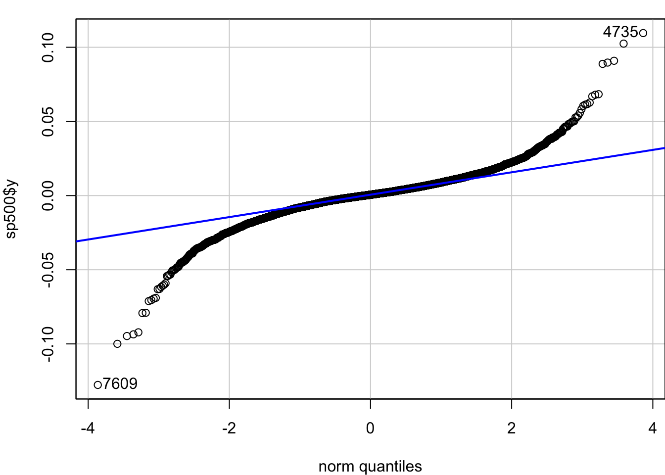
We can also use QQ-Plots to see how our data fits the distributions with various degrees of freedom.
par(mfrow=c(2,2), mar=c(4,4,1,0))
x = qqPlot(sp500$y, distribution = "norm", envelope = FALSE, xlab="normal")
x = qqPlot(sp500$y, distribution = "t", df = 4, envelope = FALSE, xlab="t(4)")
x = qqPlot(sp500$y, distribution = "t", df = 3.5, envelope = FALSE, xlab="t(3.5)")
x = qqPlot(sp500$y, distribution = "t", df = 3, envelope = FALSE, xlab="t(3)")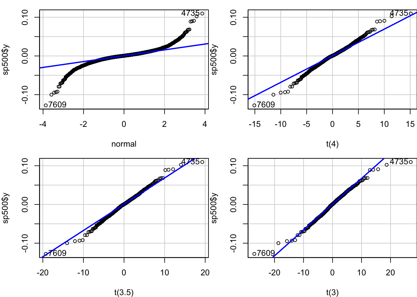
Having examined individual statistical measures and formal tests, we now turn to visualising the complete distribution of financial returns. Visual analysis complements numerical statistics by revealing patterns that summary measures might obscure, such as multimodality, unusual tail behaviour, or departures from expected distributional shapes.
The following sections demonstrate various techniques for visualising and comparing return distributions, from basic histograms to empirical distribution functions. These approaches help assess how well theoretical distributions fit actual financial data and highlight the practical implications of distributional differences across assets.
In many financial theories, returns are usually assumed to be normally distributed. In reality, stock returns are usually heavy-tailed and skewed.
To visualise the distribution of stock returns, we can use a histogram with the hist() command.
hist(sp500$y)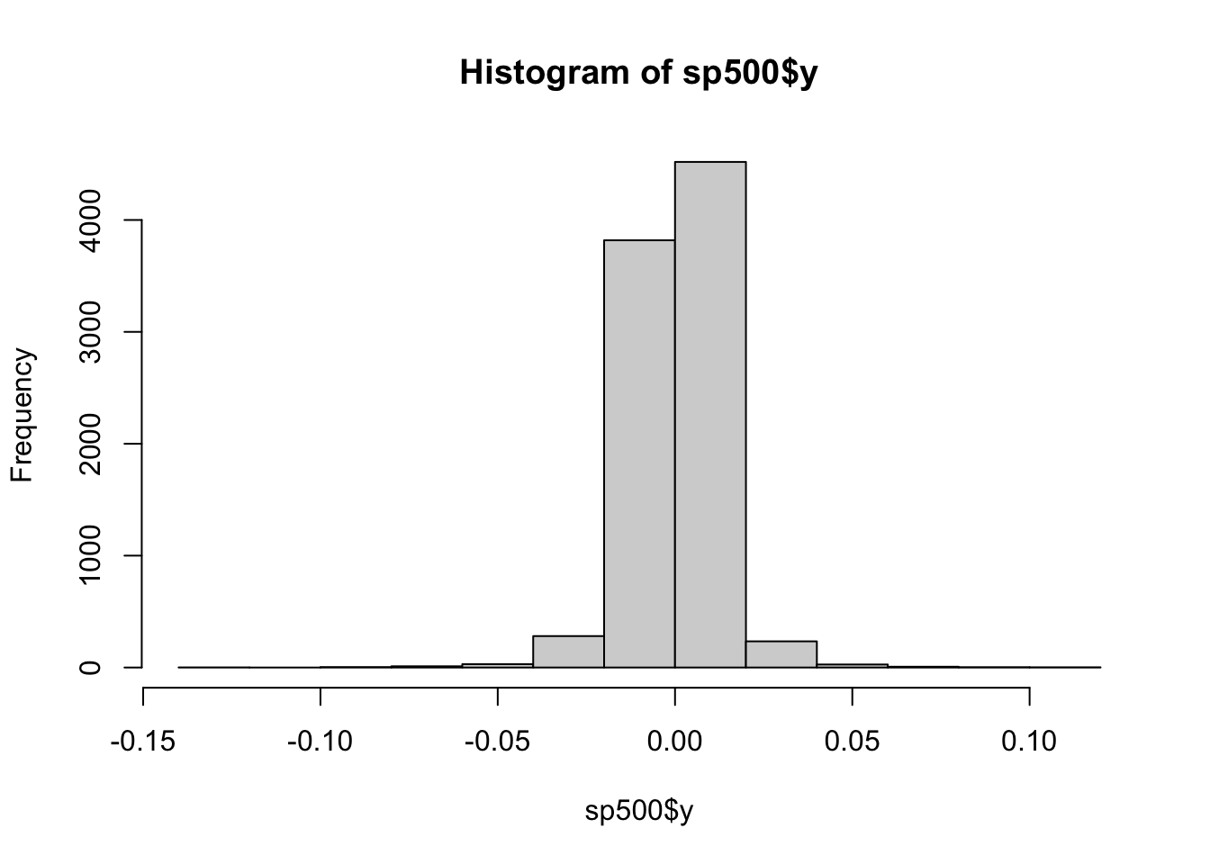
We can improve the plot a bit and superimpose the normal with the same mean and variance as the underlying data.
x = seq(min(sp500$y),max(sp500$y),length=500)
hist(sp500$y,
 freq=FALSE,
 main="S&P 500 histogram", xlab="Return",
 col= "deepskyblue3",
 breaks=30,
 las=1
)
lines(x,dnorm(x, mean(sp500$y), sd(sp500$y)), lty=2, col="red", lwd=2)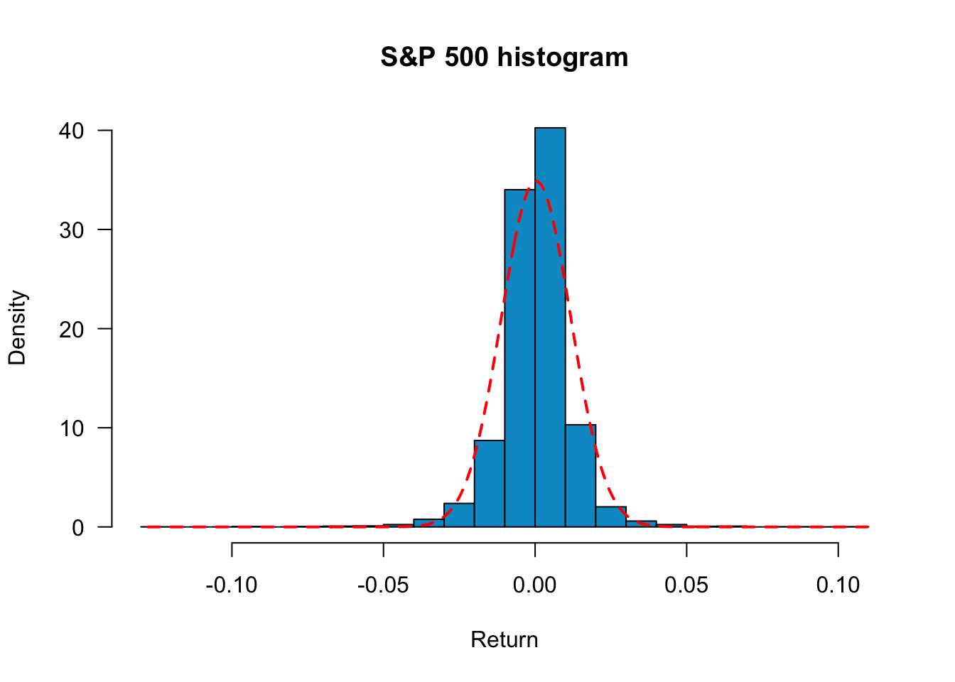
We can zoom into the plot by using xlim=c(-0.05,0.05):
hist(sp500$y,
 freq=FALSE,
 main="S&P 500 histogram", xlab="Return",
 col= "deepskyblue3",
 breaks=60,
 las=1,
 xlim=c(-0.05,0.05)
)
lines(x,dnorm(x, mean(sp500$y), sd(sp500$y)), col="red", lwd=3)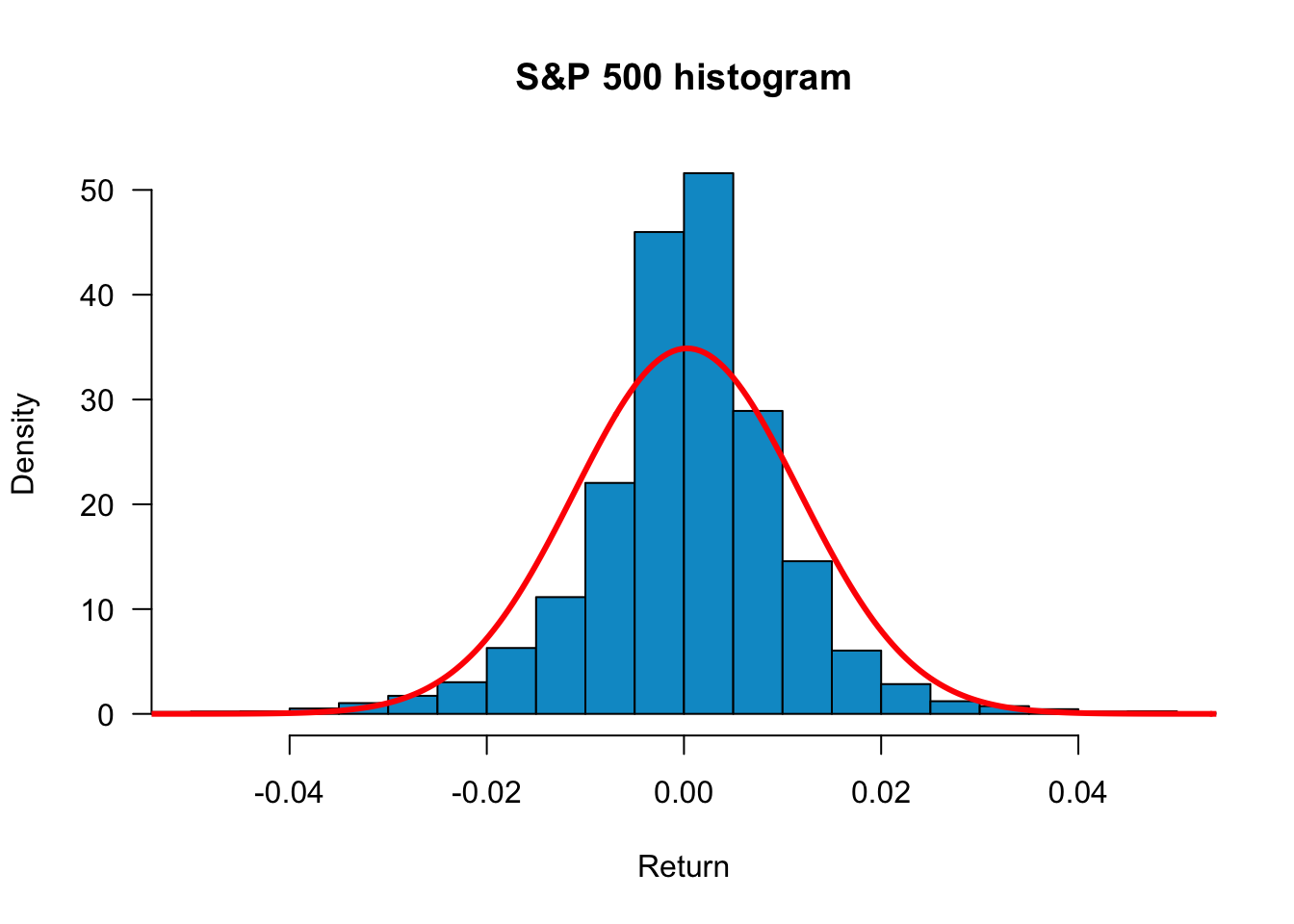
freq=F displays histograms with density instead of frequency. This is more convenient if we want to compare the empirical distributions with the normal density. main="plot_name" sets the title of the plot, and breaks=30 sets the number of bins. To add a normal density line, use the lines command. The mean and standard deviation are set to match the sample mean and sample volatility. From the plot, we see that although the empirical distribution has a bell shape, the returns have fat tails and are skewed. Returns around the mean are more frequent than the normal distribution, so S&P 500 returns appear not normally distributed.
Another way to see the return distributions is the box plot. The upper and lower edges of the box are the 75th and 25th percentile, and the thick line in the middle represents the median. All points beyond the boundary of whiskers are classified as outliers.
boxplot(sp500$y, main="Box Plot - sp500", col="deepskyblue3", ylab="Return")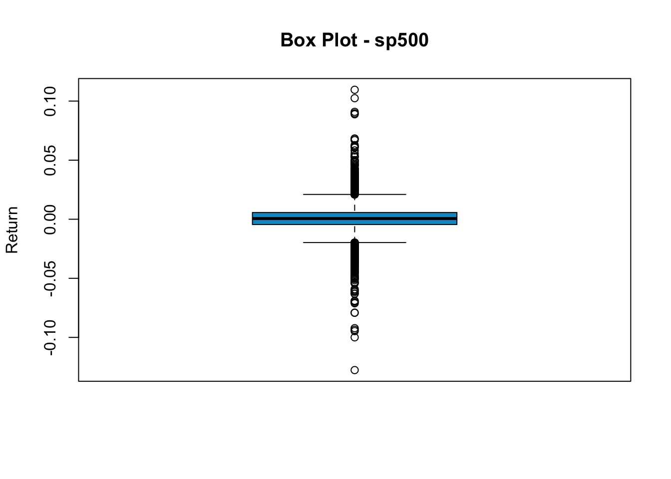
We see a significant number of outlines in sp500 returns. This indicates that unusually high/low returns are not rare. To make a horizontal box plot, add horizontal=T.
ecdf can generate the empirical cumulative distribution. Using the S&P500, we have the following plot.
plot(ecdf(sp500$y))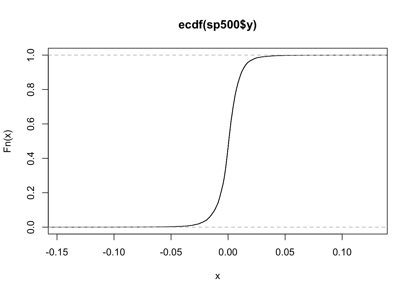
plot(ecdf(sp500$y),
 col='blue',
 main="S&P 500 empirical distribution and the normal",
 las=1,
 ylab="Probability",
 xlab="Returns"
)
x = seq(min(sp500$y),max(sp500$y),length=length(sp500$y))
lines(x,pnorm(x,mean(sp500$y),sd(sp500$y)),col='red')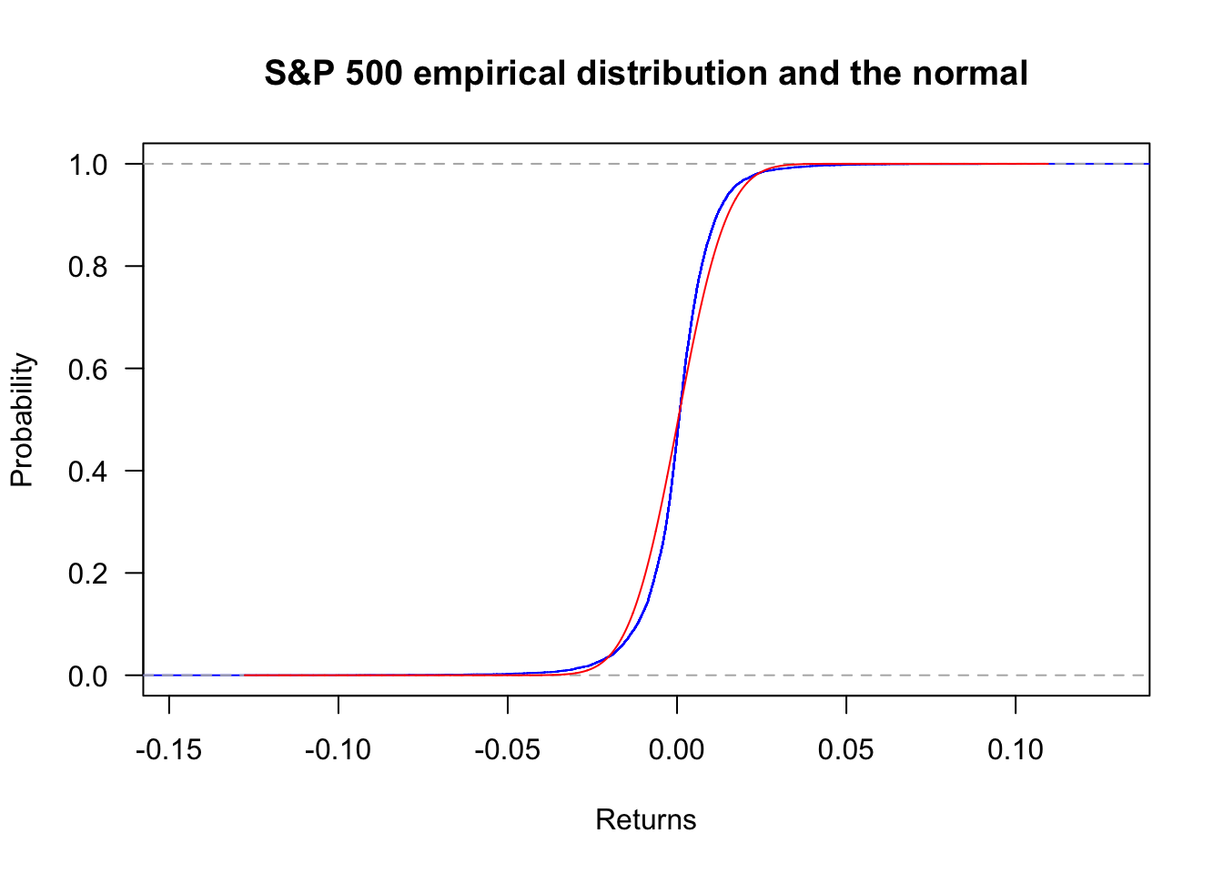
Zooming in with xlim:
plot(ecdf(sp500$y),
 col='blue',
 main="S&P 500 empirical distribution and the normal",
 las=1,
 ylab="Probability",
 xlab="Returns",
 xlim=c(-0.04,0.04)
)
x = seq(min(sp500$y),max(sp500$y),length=length(sp500$y))
lines(x,pnorm(x,mean(sp500$y),sd(sp500$y)),col='red')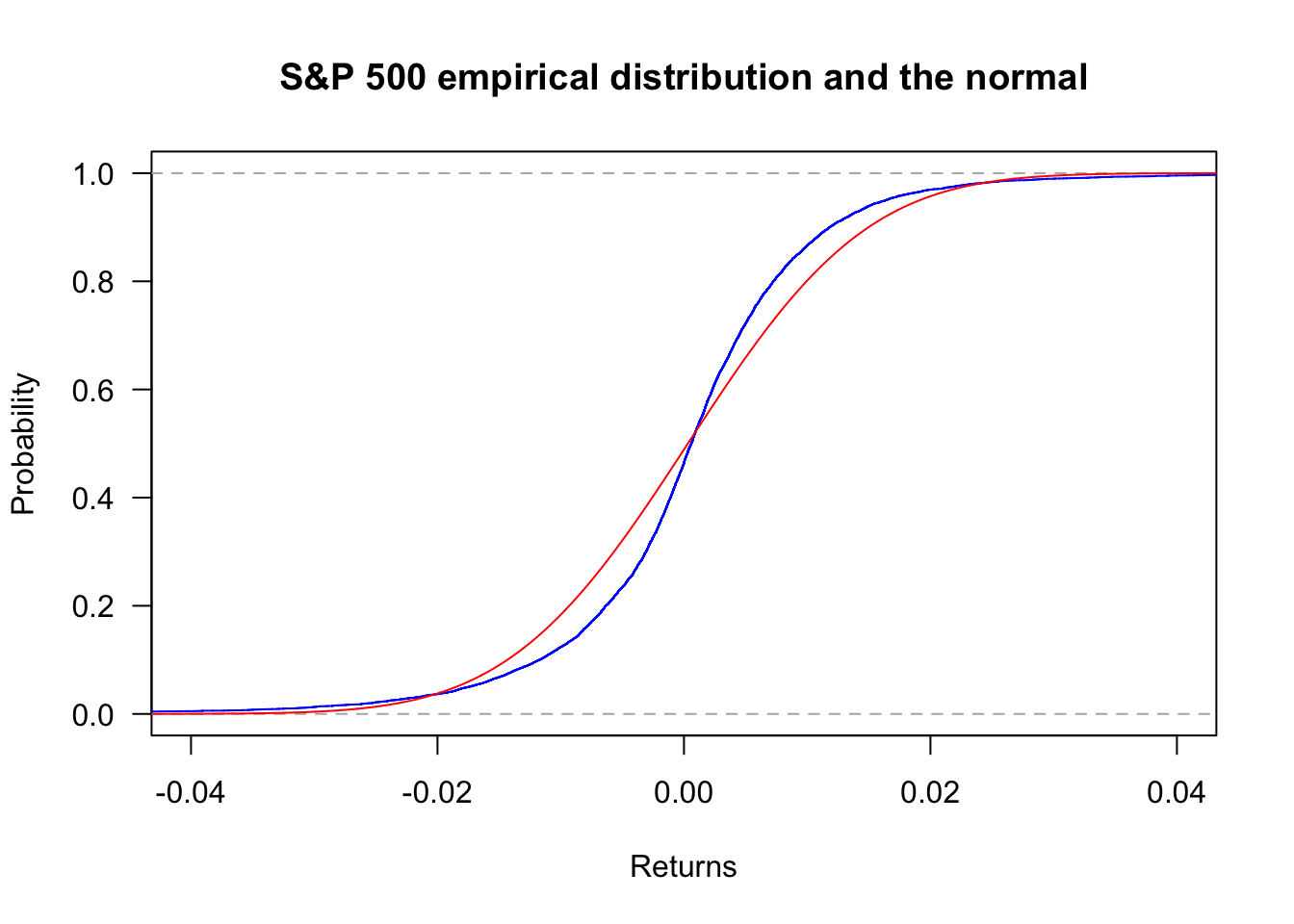
Zooming into the left tail with xlim:
plot(ecdf(sp500$y),
 col='blue',
 main="S&P 500 empirical distribution and the normal",
 las=1,
 ylab="Probability",
 xlab="Returns",
 xlim=c(-0.1,-0.03),
 ylim=c(0,0.01)
)
x = seq(min(sp500$y),max(sp500$y),length=length(sp500$y))
lines(x,pnorm(x,mean(sp500$y),sd(sp500$y)),col='red')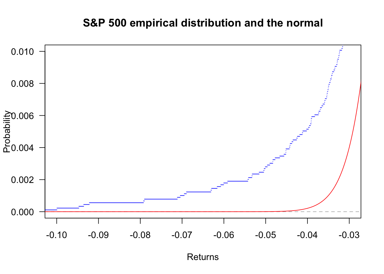
We can also compare the distribution of Apple and JPMorgan.
plot(ecdf(Return$AAPL),
     col='blue',
     las=1,
     main="Apple and JPMorgan"
)
lines(ecdf(Return$JPM),col='red')
legend('topleft', legend=c("AAPL","JPM"), col=c("blue","red"), bty='n', lty=1)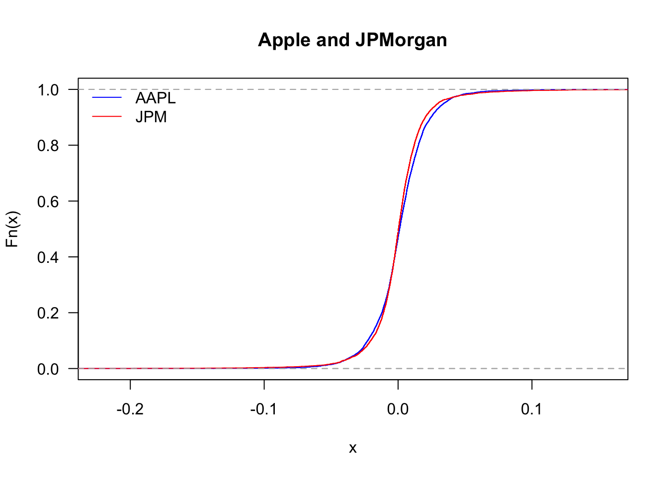
And zooming in
plot(ecdf(Return$AAPL),
     col='blue',
     xlim=c(-0.05,0.05),
     las=1,
     main="Apple and JPMorgan"
)
lines(ecdf(Return$JPM),col='red')
legend('topleft', legend=c("AAPL","JPM"), col=c("blue","red"), bty='n', lty=1)
By looking at the upper tail, we can see which of the two stocks delivers more large returns:
plot(ecdf(Return$AAPL),
     col='blue',
     xlim=c(0.02,0.1),
     ylim=c(0.83,1),
     las=1,
     main="Apple and JPMorgan"
)
lines(ecdf(Return$JPM),col='red')
legend('bottomright', legend=c("AAPL","JPM"), col=c("blue","red"), bty='n', lty=1)
The statistical analysis of financial returns reveals several important characteristics that differ markedly from normal distributions:
These findings have important implications for risk management, as models assuming normality will systematically underestimate the probability of extreme market movements.
Using data.Rdata, compute descriptive statistics for all stocks in the Return data frame. Summarise and present the results in a new data frame. It should include mean, standard deviation, skewness, kurtosis, and the p-value of the Jarque-Bera test. Keep five decimal places.