19 Multivariate volatility

Understanding how asset volatilities move together is important for portfolio risk management and derivatives pricing. Correlations change over time and spike during crises when diversification benefits disappear precisely when needed most. Multivariate models capture these dynamics for accurate portfolio VaR and optimal hedging strategies.

This chapter covers multivariate volatility implementation as discussed in chapter three of Financial Risk Forecasting. We progress from simple EWMA models through Dynamic Conditional Correlation (DCC) specifications, demonstrating how correlations evolve over time and affect portfolio risk.

GARCH models have to be solved using maximum likelihood methods. How the GARCH packages, like rmgarch, fit their models is discussed in Chapter 16. For the mathematical details, see the book or slides, and see the package documentation for how to use rmgarch.

We use maximum likelihood methods for estimating volatility models and use the R package rmgarch for the actual implementation. See the package documentation for more details, manual and a more detailed vignette. It was developed by Alexios Galanos and is regularly maintained and updated. The development code can be found on GitHub.

19.1 Data and libraries

library(reshape2)
source("common/functions.r",chdir=TRUE)
library(rmgarch)

data=ProcessRawData()
Return=data$Return
Ticker=data$Ticker

19.2 EWMA

Exponentially Weighted Moving Average (EWMA) is one of the simplest approaches to multivariate volatility modelling. Unlike sample covariance which treats all observations equally, EWMA gives more weight to recent observations, making it responsive to changing market conditions.

EWMA serves as a foundation for understanding more complex models like DCC-GARCH. It estimates the covariance matrix at time \(t\) using:

\[\Sigma_t = \lambda \times \Sigma_{t-1} + (1-\lambda) \times y_{t-1} \times y'_{t-1}\]

where \(\lambda\) is the decay parameter (typically 0.94) and \(y_t\) is the vector of returns.

The EWMA update uses matrix multiplication to compute the covariance matrix. The key operation is the outer product of returns vectors.

For a vector of returns \(y_t = [y_{1,t}, y_{2,t}]'\), the outer product \(y_t \times y_t'\) creates a matrix:

\[y_t \times y_t' = \begin{bmatrix} y_{1,t} \\ y_{2,t} \end{bmatrix} \times \begin{bmatrix} y_{1,t} & y_{2,t} \end{bmatrix} = \begin{bmatrix} y_{1,t}^2 & y_{1,t}y_{2,t} \\ y_{1,t}y_{2,t} & y_{2,t}^2 \end{bmatrix}\]

This gives us the instantaneous ‘covariance’ for that day. The diagonal elements are squared returns (variances), and off-diagonal elements are cross-products (covariances). The EWMA then weights this new information against the previous covariance matrix estimate.

We start with the special case of 2 assets to illustrate the mechanics, using JPM and Intel (INTC).

y=as.matrix(Return[,c("JPM","INTC")])
EWMA = matrix(nrow=dim(y)[1],ncol=3)
lambda = 0.94
S = cov(y)
EWMA[1,] = c(S)[c(1,4,2)]
for (i in 2:dim(y)[1]){
    S =
        lambda*S+(1-lambda)*
        y[i-1,] %*% t(y[i-1,])
    EWMA[i,] = c(S)[c(1,4,2)]
}
rhoEWMA = EWMA[,3]/sqrt(EWMA[,1]*EWMA[,2])
plot(rhoEWMA,type='l',main="EWMA Correlations for JPM and INTC")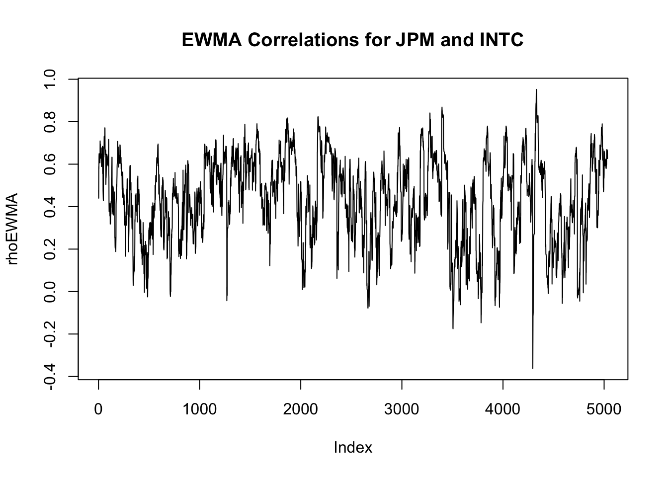

19.3 CCC and DCC

The CCC and DCC model separates volatility modelling into two stages:

Univariate stage: Each asset follows its own GARCH process for volatility;
Correlation stage: Correlations follow their own dynamic process.

This two-stage approach provides computational efficiency whilst capturing the time-varying correlation patterns useful for portfolio risk management.

19.3.1 Constant Conditional Correlation (CCC)

The Constant Conditional Correlation (CCC) model assumes that whilst individual asset volatilities change over time, the correlations between assets remain constant.

In CCC models:

Each asset follows its own univariate GARCH process for volatility;
Correlations are estimated once and held constant over time;
The covariance matrix at time \(t\) is: \(\Sigma_t = D_t R D_t\).

where \(D_t\) is a diagonal matrix of conditional standard deviations and \(R\) is the constant correlation matrix.

CCC provides a useful benchmark for evaluating whether dynamic correlations (DCC) provide significant improvements. If correlations are genuinely constant, CCC should perform as well as more complex models.

19.3.2 Dynamic Conditional Correlation (DCC)

Dynamic Conditional Correlation (DCC) models extend the CCC framework by allowing correlations to vary over time whilst maintaining the flexibility of GARCH specifications for individual asset volatilities. Unlike constant correlation models, DCC captures how correlations spike during market stress and evolve with changing market conditions.

The DCC model separates volatility modelling into two stages:

Univariate stage: Each asset follows its own GARCH process for volatility;
Correlation stage: Correlations follow their own dynamic process, similar to GARCH but for correlation matrices.

This two-stage approach provides computational efficiency whilst capturing the time-varying correlation patterns useful for portfolio risk management.

19.4 `rmgarch`

The package rmgarch allows us to estimate models with multiple assets in the same fashion as rugarch. The procedure is analogous: We first need to specify the model we want to use and then fit it to the data. However, specifying the model requires additional steps. To explain this, we will focus on the estimation of a DCC model.

In a DCC model, we assume that each asset follows some univariate model, usually a GARCH. Then, we model the correlation between the assets using an ARMA-like process.

The process for fitting a DCC model using rmgarch is:

Specify the univariate volatility model each asset follows using ugarchspec();
Use the multispec() function to create a multivariate specification. This is a list of univariate specifications. If we are going to use the same specification for every asset, we can use replicate();
Create a dccspec() object, which takes the list of univariate specifications for every asset and the additional DCC joint specifications, like dccOrder and distribution;
Fit the specification to the data.

We will use the returns for JPM and Intel (INTC):

y=as.matrix(Return[,c("JPM","INTC")])

We will assume a simple normal GARCH(1,1) with zero mean for each stock individually. We will create a single univariate specification and then replicate it using multispec():

# Create the univariate specification
uni_spec = ugarchspec(
    variance.model = list(
        garchOrder = c(1,1)),
        mean.model = list(
        armaOrder = c(0,0),
        include.mean = FALSE
    )
)
# Replicate it into a multispec element
mspec = multispec(replicate(2, uni_spec))

Examine the mspec object. We will see there are two univariate specifications, one per asset, and they are identical:

mspec


*-----------------------------*
*     GARCH Multi-Spec        *
*-----------------------------*
Multiple Specifications : 2
Multi-Spec Type         : equal

You can check the specifications with mspec@spec.

Now we proceed to create the specification for the DCC model using dccspec():

spec = dccspec(
 # Univariate specifications - Needs to be multispec
 uspec = mspec,

 # DCC specification. We will assume an ARMA(1,1)-like process
 dccOrder = c(1,1),

 # Distribution, here multivariate normal
 distribution = "mvnorm"
)

We can call spec to see what is inside:

spec


*------------------------------*
*       DCC GARCH Spec         *
*------------------------------*
Model          :  DCC(1,1)
Estimation     :  2-step
Distribution   :  mvnorm
No. Parameters :  9
No. Series     :  2

We can again see more details in spec@model and spec@umodel.

Now we can proceed to fit the specification to the data:

res = dccfit(spec, data = y)
res


*---------------------------------*
*          DCC GARCH Fit          *
*---------------------------------*

Distribution         :  mvnorm
Model                :  DCC(1,1)
No. Parameters       :  9
[VAR GARCH DCC UncQ] : [0+6+2+1]
No. Series           :  2
No. Obs.             :  5034
Log-Likelihood       :  27227.76
Av.Log-Likelihood    :  5.41 

Optimal Parameters
-----------------------------------
               Estimate  Std. Error  t value Pr(>|t|)
[JPM].omega    0.000004    0.000003   1.5612  0.11847
[JPM].alpha1   0.092327    0.017140   5.3867  0.00000
[JPM].beta1    0.896337    0.020491  43.7422  0.00000
[INTC].omega   0.000004    0.000003   1.3602  0.17377
[INTC].alpha1  0.030623    0.004387   6.9801  0.00000
[INTC].beta1   0.959937    0.001737 552.5942  0.00000
[Joint]dcca1   0.009528    0.005875   1.6219  0.10483
[Joint]dccb1   0.973321    0.020500  47.4799  0.00000

Information Criteria
---------------------
                    
Akaike       -10.814
Bayes        -10.802
Shibata      -10.814
Hannan-Quinn -10.810


Elapsed time : 1.006636

We can check what slots are inside:

names(res@model)

 [1] "modelinc"      "modeldesc"     "modeldata"     "varmodel"     
 [5] "pars"          "start.pars"    "fixed.pars"    "maxgarchOrder"
 [9] "maxdccOrder"   "pos.matrix"    "pidx"          "DCC"          
[13] "mu"            "residuals"     "sigma"         "mpars"        
[17] "ipars"         "midx"          "eidx"          "umodel"

names(res@mfit)

 [1] "coef"            "matcoef"         "garchnames"      "dccnames"       
 [5] "cvar"            "scores"          "R"               "H"              
 [9] "Q"               "stdresid"        "llh"             "log.likelihoods"
[13] "timer"           "convergence"     "Nbar"            "Qbar"           
[17] "plik"

# Coefficient matrix
res@mfit$matcoef

                  Estimate   Std. Error    t value     Pr(>|t|)
[JPM].omega   4.320439e-06 2.767316e-06   1.561238 1.184676e-01
[JPM].alpha1  9.232660e-02 1.713985e-02   5.386662 7.177819e-08
[JPM].beta1   8.963372e-01 2.049136e-02  43.742208 0.000000e+00
[INTC].omega  3.501042e-06 2.573931e-06   1.360193 1.737689e-01
[INTC].alpha1 3.062283e-02 4.387153e-03   6.980115 2.949418e-12
[INTC].beta1  9.599367e-01 1.737146e-03 552.594221 0.000000e+00
[Joint]dcca1  9.528054e-03 5.874660e-03   1.621890 1.048268e-01
[Joint]dccb1  9.733205e-01 2.049965e-02  47.479853 0.000000e+00

# Log likelihood
res@mfit$llh

[1] 27227.76

The matrix H inside res@mfit includes the covariances. It is 3-dimensional, since it includes the 2x2 covariance matrix for each of the T time periods:

H = res@mfit$H
dim(H)

[1]    2    2 5034

# First period's covariances
H[,,1]

             [,1]         [,2]
[1,] 0.0005220625 0.0001946884
[2,] 0.0001946884 0.0003907303

We can extract the conditional correlation in two ways. One is computing it from H:

# Initializing the vector
rhoDCC = vector(length = dim(y)[1])

# Populate with the correlations
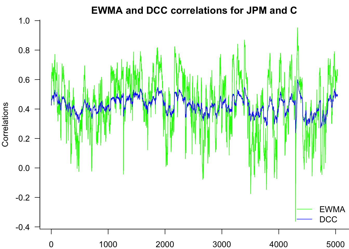
rhoDCC = H[1,2,] / sqrt(H[1,1,]*H[2,2,])

19.5 Compare EWMA and DCC

par(mar=c(2,4,2,0))
matplot(cbind(rhoEWMA,rhoDCC),
 type='l',
 bty='l',
 lty=1,
 col=c("green","blue"),
 main="EWMA and DCC correlations for JPM and C",
 ylab="Correlations",
 las=1
)
legend("bottomright",
 legend=c("EWMA","DCC"),
 lty=1,
 col=c("green","blue"),
 bty='n'
)

19.6 Exercise

Following the steps specified in the slides, construct the conditional variance matrix for JPM and INTEL using the constant conditional correlations (CCC) model and compute the constant conditional correlation.