22 Running Backtests

Backtesting requires the systematic generation of risk forecasts using historical data. Having developed VaR models in Chapter 20, we now need computational infrastructure to apply these models across thousands of trading days to generate the data required for subsequent validation.

This chapter focuses on the computational implementation of backtesting:

Framework setup: Establishing consistent parameters and data structures for systematic testing;
Performance optimisation: Using parallel processing to handle computationally intensive GARCH models;
Data management: Generating comprehensive datasets with forecasts, actual returns, and dates;
Platform compatibility: Implementing solutions for both Unix and Windows systems;
Reproducibility: Creating caching systems to ensure consistent results across runs.

The goal is to transform individual risk models into a systematic forecasting framework that can process large datasets efficiently. This generates the comprehensive backtesting dataset needed for statistical validation.

Building on the risk forecasting methods from Chapter 20, and using functions.r from there, we implement the computational infrastructure to run these models systematically across historical data.

The next chapter, Chapter 23, uses this generated data to perform statistical validation of model performance.

22.1 Data and libraries

We load the necessary packages for backtesting analysis, including libraries for data manipulation, parallel processing, and performance measurement.

library(reshape2)
library(zoo)
library(rugarch)
library(microbenchmark)
library(parallel)
library(foreach)
library(iterators)
library(doParallel)
library(digest)
source("common/functions.r",chdir=TRUE)

microbenchmark is to evaluate execution speed;
parallel, foreach, iterators and doParallel are used for multicore (parallel) execution.

data = ProcessRawData()
sp500 = data$sp500

22.2 Backtesting framework setup

We establish consistent parameters for systematic backtesting across all risk models. The parameter structure ensures fair comparison and reproducible results.

par        = list()
par$p      = 0.01        # probability level (5% VaR)
par$value  = 1000        # portfolio value in currency units
par$WE     = 2000        # estimation window size
par$T      = length(sp500$y)  # total sample size
par$WT     = par$T-par$WE     # testing window size
par$lambda = 0.94         # decay parameter for EWMA
par$Methods = c("HS","EWMA","GARCH","tGARCH") # models we run

22.3 Intermediate files consideration

We argued in Section Section 15.2 that we should normally avoid intermediate files unless strictly necessary. Backtesting might provide the exception. The reason is that the time to estimate some of the models we use is not trivial. When we have to repeat the estimation every day in the testing window, the estimation time can become excessive. Since we then have to process the backtesting results, it may be more efficient to run them in a separate file, save them, and then code up the processing separately.

That said, it might be sensible to do that when developing the code that reports on the backtest, but it would usually be best not to create intermediate files for the final run.

22.4 Backtesting functions

Systematic backtesting requires a structured approach to ensure consistent methodology across different risk models and time periods. We implement this through two complementary functions that separate daily forecast generation from the overall backtesting framework.

The two-function design serves several purposes:

Modularity: RunOneDay() handles individual forecast generation, making it easy to test and debug single-day calculations
Flexibility: The same daily function works with different risk models through dynamic function calling
Performance measurement: Separating functions allows us to benchmark individual model execution times
Parallel processing: The modular structure enables efficient multi-core implementation for computationally intensive models

This systematic approach ensures that each risk model (HS, EWMA, GARCH, t-GARCH) receives identical treatment during backtesting, providing fair comparison of their forecasting performance.

We divided the code to run the backtesting into two functions, RunOneDay() and Backtesting(). While not strictly necessary, this separation of functionality is helpful in our case because we want to evaluate the time it takes to do the backtesting.

22.4.1 `RunOneDay()`

Note the line

#| eval: false
x=do.call(
  what=paste0("Risk.",par$Methods[i]),
  args=...
)

in function RunOneDay(). Here, paste0("Risk.",par$Methods[i]) just takes an estimation method and combines it with the string Risk. For example, if par$Methods[i] is HS, we get Risk.HS, which is one of the risk functions we use.

do.call(what) then calls the function in the what argument, in this case Risk.HS() with arguments y=sp500$y[t1:t2],par=par,Print=Print.

Note that the vector res holds both the VaR and ES results. The reason we do it that way is to facilitate the multi-core implementation below.

If we call RunOneDay() with HeaderOnly=TRUE, it returns headers, or labels, for the data it otherwise genertes, useful for creating a datraframe below.

RunOneDay=function(t=NULL,y=NULL,Methods,Print=FALSE,HeaderOnly=FALSE)  {
  if(HeaderOnly) {
    header=c()
    for(i in 1:length(Methods)){
      header[i]=paste0("VaR.",Methods[i])
      header[i+length(Methods)]=paste0("ES.",Methods[i])
    }
    header=c(header,"index","y")
    return(header)
  }
  t2 = t-1
  t1 = t2-par$WE+1
  if(Print) cat(t,t2,t1,"\n")
  res = rep(0,2*length(Methods))
    for(i in 1:length(Methods)){
    x = do.call(what=paste0("Risk.",Methods[i]),args=list(y=y[t1:t2],par=par,Print=Print ))
    res[i] = x$VaR
    res[i+length(Methods)] = x$ES

  }
  res=c(res,t)
  res=c(res,y[t])

  return(res)
}

22.5 How long does it take to run?

Backtesting is slow, except for the fastest methods. There are several ways to measure the time it takes to run an R command. The easiest is to take note of Sys.time(), which measures the actual time it is run. We can then run some code and compare the changes in Sys.time(). This is sometimes known as wall time because it measures the time a wall clock would take. The benefit is that this approach is straightforward.

The downside is that many factors can affect how long the code takes. The computer might be doing something else at the same time, which affects the results. Often, if we call the same function repeatedly, the first call takes the longest time, as we see here.

A more accurate method is to repeat the run several times and use the minimum or median value. The easiest way to do that is with the R command microbenchmark().

22.5.1 Wall time

  time1 = Sys.time()
  res = RunOneDay(par$T,y=sp500$y,Methods=c("HS"))
  print(Sys.time() -time1)

Time difference of 0.008721828 secs

  time1 = Sys.time()
  res = RunOneDay(par$T,y=sp500$y,Methods=c("EWMA"))
  print(Sys.time() -time1)

Time difference of 0.004758835 secs

  time1 = Sys.time()
  res = RunOneDay(par$T,y=sp500$y,Methods=c("GARCH"))
  print(Sys.time() -time1)

Time difference of 0.05553889 secs

  time1 = Sys.time()
  res = RunOneDay(par$T,y=sp500$y,Methods=c("tGARCH"))
  print(Sys.time() -time1)

Time difference of 0.206527 secs

22.5.2 With `microbenchmark`

Start by running the microbenchmark for a GARCH model. In this case, it reports the results in milliseconds or one-thousandth of a second.

m = microbenchmark(
  RunOneDay(par$T,y=sp500$y,Methods=c("GARCH"))
)
m$expr = "GARCH"
print(m)

Unit: milliseconds
  expr      min       lq     mean   median      uq      max neval
 GARCH 31.43462 32.59043 37.20961 33.97932 35.3158 107.7191   100

If we want to compare several methods, it is best to collect the output from microbenchmark in a vector. Note that the raw output is measured in nanoseconds or one billionth of a second.

  res = vector(length=length(par$Methods))
  for(i in 1:length(par$Methods)){
    m = microbenchmark(
      RunOneDay(par$T,y=sp500$y,Methods=par$Methods[i])
    )
    res[i] = summary(m, unit = "ms")$median
  }
  print(res)

[1]  0.0489335  0.3208045 34.6492845 62.3787940

We can then plot them together, in this case, with a bar plot. Since the numbers are very different, a log scale helps.

a = barplot(res,
  log='y',
  las=1,
  border=FALSE,
  ylab="Milliseconds",
  names.arg=par$Methods,
  main="Milliseconds",
  col="lightblue"
)
text(a,res*1.17,round(res,2),xpd=TRUE)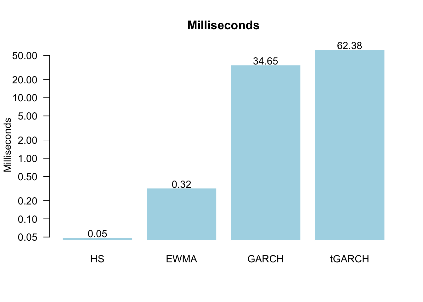

While 0.06 seconds for tGARCH does not seem that long when repeated 6938 times over the testing window, it ends up taking 7.2 minutes.

22.6 Sequential backtesting baseline

Before exploring parallel solutions, we could establish how long a complete sequential backtest takes and why this becomes problematic for practical risk management. But it takes too long.

time_sequential = proc.time()
sequential_results = lapply(
        (par$WE+1):par$T,
        RunOneDay,
        y=sp500$y,
        Methods=par$Methods
    )
time_sequential = proc.time() - time_sequential
print(paste("Sequential backtest time:", round(time_sequential["elapsed"]/60, 2), "minutes"))

For 6938 trading days with 4 methods, sequential processing requires significant time, particularly with GARCH models that involve numerical optimisation at each step.

This timing constraint becomes problematic for risk managers who need:

Daily model recalibration and validation
Multiple scenario testing
Regulatory reporting deadlines
Real-time risk monitoring capabilities

22.7 Parallel processing solution

Having established the baseline performance constraints, parallel processing provides a natural solution. Each day’s forecast is independent of others within the rolling window framework, making backtesting well-suited for multi-core implementation.

The performance benefits can be considerable: if your computer has multiple cores, your backtesting job may run several times faster. This can transform the lengthy sequential process into a more manageable task, enabling broader model evaluation.

22.7.1 Available processing power

Modern computers typically have multiple cores available. By default, R uses only one core, but most computers have at least 4 cores, and some laptops have 16 or more.

Two considerations arise when running jobs on multiple cores.

The first is that it is inevitably more complex. You need to write your code in a way that makes it easy for it to run on multiple cores and then call a special function actually to do that.

The second problem is that running multiple cores has some overhead, so small jobs can take longer to run on multiple cores than a single one.

22.7.2 Implementation approach

Parallel backtesting relies on R’s Apply family of functions, which provide the foundation for distributing our daily risk calculations across multiple processor cores. These functions are useful because they automatically handle the process of applying our RunOneDay() function to each trading day in the testing window.

The Apply family works well for backtesting because:

Vector processing: Each element of our date vector (par$WE+1):par$T gets processed independently;
Function application: The same RunOneDay() function runs on each trading day;
Result aggregation: Output from each day gets collected into a structured list;
Parallel scaling: Multi-core versions (mclapply()) distribute work automatically.

This is why we designed RunOneDay() to return a vector rather than a list — it ensures the parallel processing functions can efficiently combine results from all trading days into our final backtesting matrix.

The technical details of apply functions are well-documented online, but for backtesting, the important point is that each day’s VaR calculation is independent, making parallel processing both practical and useful.

22.7.3 System requirements and setup

It can be useful to identify your computer’s processing capacity for backtesting optimisation. Different computers have varying numbers of cores, and checking this automatically helps ensure our parallel processing makes good use of available resources.

cores = detectCores()

The computer we are now using has 10 cores.

22.7.4 Platform differences

We have an issue that arises because of differences between Windows computers and UNIX, which includes Macs and Linux. The way R does multi-core processing is more efficient on UNIX computers through forking, whilst Windows requires cluster-based approaches.

We will use mclapply() on Mac and Linux and foreach() on Windows. Both work on Mac and Linux, but Windows cannot use mclapply().

mclapply() needs library(parallel)
foreach() needs library(foreach) and library(doParallel)

22.7.5 Result ordering considerations

When using parallel processing functions, there is a consideration about result ordering that matters for backtesting. The parallel processing may optimise job distribution rather than simply splitting work sequentially. While this does not matter for some applications like Monte Carlo simulations, it is worth noting for backtesting since we need to match risk forecasts to specific trading days. We therefore take care below to ensure proper ordering.

22.8 Mac/Linux — `mclapply()`

The mclapply() function accepts several arguments:

mclapply(
  X,              # vector or list to iterate over
  FUN,            # function to apply to each element
  ...,            # additional arguments passed to FUN
  mc.cores,       # number of processor cores to use
  mc.preschedule  # controls job scheduling across workers
)

In our backtesting context, this becomes: - X = setup$range: the vector of trading days to process - FUN = RunOneDay: the function calculating VaR and ES for each day - ...: additional arguments like y=setup$y, Methods=par$Methods - mc.cores = cores: uses all available processor cores - mc.preschedule = TRUE: ensures results maintain chronological order

If we don’t specify parallel parameters, mclapply() simply becomes lapply() running on a single core.

We could run the parallel version directly like:

#| eval: false
time1 = proc.time()
res1 = mclapply(
  (par$WE+1):par$T,
  RunOneDay,
  y=sp500$y,
  mc.cores=cores,
  mc.preschedule=TRUE
)
time1 = proc.time()-time1
print(time1)
print(res1[1:2])

This uses all available cores (mc.cores=cores) and maintains chronological order (mc.preschedule=TRUE). However, running this calculation repeatedly during development becomes inefficient, particularly with computationally intensive GARCH models. When the data and parameters are unchanged, we can use the idea from Section Section 15.4.2.2 and hash the output to avoid redundant calculations. The setup structure captures all this information for the caching system.

We implement the caching system by creating a comprehensive setup structure that captures all the relevant inputs for our backtesting run. This includes the data, the range of dates to process, the methods to test, and all parameters. We then generate a unique filename using a cryptographic hash of this setup, ensuring that any change to the inputs will create a different cache file:

setup=list(
  y=sp500$y,
  range=(par$WE+1):par$T,
  Methods=par$Methods,
  date=sp500$date,
  par=par
)
file_name=paste0(digest(setup),".RData")
cat(file_name,"\n")

c7ef19181b210818a08827a5364acc5d.RData

The digest function plays a key role by creating a unique fingerprint from the setup contents. This cryptographic hash ensures that any change to the data, parameters, date range, or methods will generate a different filename, automatically invalidating the cache when inputs change whilst preserving results when they remain constant.

With the caching system established, we can now implement the conditional execution that either loads existing results or performs the parallel calculation.

A key consideration is if date indices will match.

time1 = proc.time()
if (file.exists(file_name)) {
  load(file_name)

} else {
    message("Running")
  backtest = mclapply(
    setup$range,
    RunOneDay,
    y=setup$y,
    Methods=par$Methods,
    mc.cores=cores,
    mc.preschedule=TRUE
  )
  class(backtest)
  backtest= data.frame(do.call(rbind, backtest))
  class(backtest)
  names(backtest)=RunOneDay(Methods=par$Methods,HeaderOnly=TRUE)
  backtest$date=setup$date[backtest$index]
  backtest$date.t=ymd(backtest$date)
  save(backtest,file=file_name)
}
print(head(backtest,2))

    VaR.HS VaR.EWMA VaR.GARCH VaR.tGARCH    ES.HS  ES.EWMA ES.GARCH ES.tGARCH
1 21.24883 37.36930  35.31112    39.4467 28.14014 42.81269 40.45470  51.04920
2 21.24883 36.23421  34.69503    38.7129 28.14014 41.51225 39.74887  50.09264
  index           y     date     date.t
1  2001 0.003943289 19971128 1997-11-28
2  2002 0.020071445 19971201 1997-12-01

print(tail(backtest,2))

       VaR.HS VaR.EWMA VaR.GARCH VaR.tGARCH  ES.HS  ES.EWMA ES.GARCH ES.tGARCH
6937 35.75759 24.05983  18.67771   20.67565 53.328 27.56450 21.39839  26.74528
6938 35.75759 23.76685  17.92987   19.84199 53.328 27.22884 20.54161  25.66556
     index           y     date     date.t
6937  8937 0.005205431 20250627 2025-06-27
6938  8938 0.005151078 20250630 2025-06-30

print(proc.time()-time1)

   user  system elapsed 
  0.003   0.001   0.004

And to quickly verify it is OK.

plot(backtest$date.t,1000*backtest$y,type='l')
lines(backtest$date.t,-backtest$VaR.EWMA,col="red",lwd=2)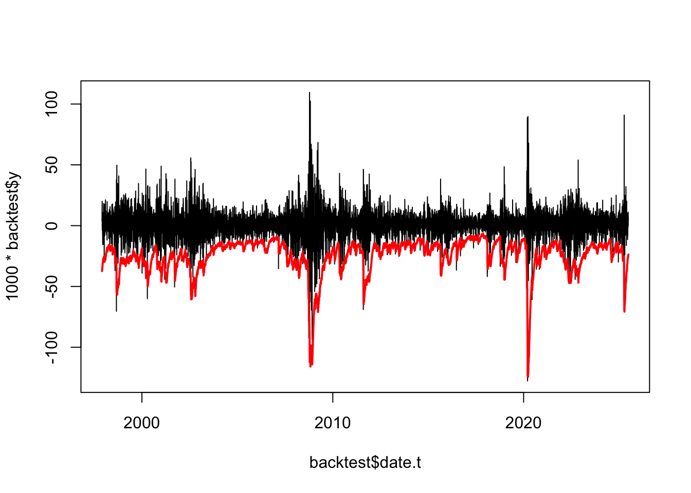

The mclapply() call uses mc.cores=cores to utilise all 10 available processor cores, and mc.preschedule=TRUE to ensure the results maintain chronological order across the parallel workers.

The mclapply() function returns a list where each element contains the VaR and ES results from RunOneDay() for one trading day. Since RunOneDay() returns a vector of length 2*length(Methods) (VaR values followed by ES values), the resulting backtest list has the same structure as if we had used lapply() sequentially.

We then transform this list into a data frame using do.call(rbind, backtest), which combines all the daily result vectors into a matrix with one row per trading day. This works because each element of the list has the same length and structure.

The data transformation process involves several steps: 1. backtest = data.frame(do.call(rbind, backtest)) converts the list into a data frame where each row represents one trading day and each column represents one risk measure (VaR or ES) for one method. 2. names(backtest) = RunOneDay(Methods=par$Methods,HeaderOnly=TRUE) sets appropriate column names by calling RunOneDay() with HeaderOnly=TRUE, which returns descriptive names like “VaR.HS”, “VaR.EWMA”, “ES.HS”, “ES.EWMA” without needing to perform any calculations. 3. backtest$y = setup$y[setup$range] adds the actual returns for each trading day to enable comparison between forecasted risk and realised outcomes. 4. backtest$date = setup$date[setup$range] adds the corresponding dates to make the results easier to interpret and analyse.

The final backtest data frame contains all the information needed for backtesting analysis: risk forecasts, actual returns, and dates.

22.8.1 Performance considerations

While parallel processing provides significant speedup, the multicore implementation is not quite 10 times faster than sequential processing. There is considerable overhead associated with distributing work across cores and combining results.

22.9 Windows (and Mac/Linux)

While the Mac/Linux approach uses efficient forking mechanisms, Windows requires a different parallel processing strategy. Windows cannot use mclapply() due to operating system limitations, necessitating a cluster-based approach that explicitly manages multiple R processes.

We use the same setup and file_name defined in the Mac/Linux section above for consistent caching.

The cluster-based approach is more complex than forking. We must create a cluster and then provide each worker with copies of all required packages, functions, and data.

The variable cl is the cluster we make:

#| eval: false
cl = makeCluster(cores)
registerDoParallel(cl)

Each worker process starts with a clean environment, so we must explicitly provide all required components:

Loading packages and functions: clusterEvalQ() executes code on each worker to load the necessary libraries and source our custom functions:

x=clusterEvalQ(cl, {
  library(reshape2)
  library(rugarch)
  library(lubridate)
  library(zoo)
  source("common/functions.r",chdir=TRUE)
})

Exporting data: clusterExport() copies specific variables from the master process to each worker:

#| eval: false
clusterExport(cl,c("par", "y","Methods"))

Running the parallel computation: With the cluster prepared, we use foreach() with the %dopar% operator to distribute work:

#| eval: false
res3=foreach(i = (par$WE+1):par$T) %dopar% {
  RunOneDay(i,y=y,Methods=par$Methods)
}

Cleaning up: Always destroy the cluster to free system resources:

#| eval: false
stopCluster(cl)

These individual components combine into the complete implementation shown below, which also incorporates the same caching mechanism used in the Mac/Linux version:

time3 = proc.time()
if (file.exists(file_name)) {
  load(file_name)
  message("File found")
} else {
  message("Running")
  cl = makeCluster(cores)
  registerDoParallel(cl)

  x = clusterEvalQ(cl, {
    library(reshape2)
    suppressPackageStartupMessages(library(rugarch))
    suppressPackageStartupMessages(library(lubridate))
    suppressPackageStartupMessages(library(zoo))
    source("common/functions.r",chdir=TRUE)
  })

  clusterExport(cl,c("par", "setup"))

  backtest = foreach(i = setup$range) %dopar% {
    RunOneDay(i,y=setup$y,Methods=par$Methods)
  }
  stopCluster(cl)
  backtest = data.frame(do.call(rbind, backtest))
  names(backtest) = RunOneDay(Methods=par$Methods,HeaderOnly=TRUE)
  backtest$date=setup$date[backtest$index]
  save(backtest,file=file_name)
}
time3 = proc.time()-time3
print(time3)
print(head(backtest))

22.9.1 Implementation comparison

The Windows cluster implementation mirrors the Mac/Linux approach in structure but differs in execution mechanics:

Similarities: Both use the same caching system, produce identical data structures, and apply the same data transformations. The foreach() %dopar% construct returns a list with the same structure as mclapply() - each element contains the VaR and ES results from RunOneDay() for one trading day. Despite using different parallel processing mechanisms (Unix forking vs Windows clusters), both approaches produce equivalent list structures that can be processed identically in the subsequent data transformation steps.

Like the Mac/Linux version, we transform this list into a data frame using do.call(rbind, backtest) to combine all daily results into a matrix format.

The final backtest data frame contains all the information needed for backtesting analysis: risk forecasts, actual returns, and dates.

22.10 Next steps

Having implemented parallel backtesting frameworks for both Unix and Windows systems, we now have the computational infrastructure to generate VaR and ES forecasts across thousands of trading days. The backtest data frame contains our risk forecasts alongside actual returns and dates, providing a foundation for systematic model evaluation.

The question remains: how do we determine whether our risk models are performing adequately? This requires statistical testing of the backtesting results to validate model accuracy and compare performance across different approaches.

The next chapter, Chapter 23, implements statistical tests for backtesting validation, including:

Violation frequency analysis to test if VaR exceedances occur at expected rates;
Independence testing to check if violations are clustered;
Comparative analysis across HS, EWMA, GARCH, and t-GARCH models
Regulatory compliance metrics for Basel framework requirements.

These tests help transform our computational results into insights for risk management practice.

22.1 Data and libraries

22.2 Backtesting framework setup

22.3 Intermediate files consideration

22.4 Backtesting functions

22.4.1 RunOneDay()

22.5 How long does it take to run?

22.5.1 Wall time

22.5.2 With microbenchmark

22.6 Sequential backtesting baseline

22.7 Parallel processing solution

22.7.1 Available processing power

22.7.2 Implementation approach

22.7.3 System requirements and setup

22.7.4 Platform differences

22.7.5 Result ordering considerations

22.8 Mac/Linux — mclapply()

22.8.1 Performance considerations

22.9 Windows (and Mac/Linux)

22.9.1 Implementation comparison

22.10 Next steps

22.4.1 `RunOneDay()`

22.5.2 With `microbenchmark`

22.8 Mac/Linux — `mclapply()`