library(reshape2)
library(lubridate)
library(zoo)
library(xts)
library(tseries)
library(ggplot2)
library(moments)
source("common/functions.r", chdir = TRUE)17 Presentations and reports
A risk analyst submits a VaR report to the regulator on Friday. On Monday, the regulator asks for the same analysis with an updated dataset. If the original report was assembled by hand — copying numbers from a console, pasting charts into slides — recreating it takes hours and invites transcription errors. A reproducible report, where code and narrative live in a single source file, regenerates in seconds with the new data, keeping every number and chart consistent with it.
There are two main approaches to creating reports from data analysis. One is the traditional copy-and-paste method using familiar software. The other is an integrated reporting system that combines code and output directly.
Many integrated approaches are based on Markdown, a lightweight markup language that uses plain text formatting syntax. Unlike Word’s complex formatting system, Markdown files are readable as plain text and can be easily version-controlled. Quarto is a publishing system built around Markdown that works well with R, Python and Julia, allowing us to embed our analysis directly into reports. This ensures that calculations, plots and statistics are consistent with the underlying data, reducing errors from manual copying and making it easier to update reports when new data arrives.
17.1 Data and libraries
The data below is what the example reports are built from.
data = ProcessRawData()

Prices = tail(data$Price, 500)
Returns = tail(data$Return, 500)
tickers = names(Returns)[2:length(names(Returns))]
import pandas as pd
import numpy as np
from scipy import stats
from scipy.stats import skew, kurtosis, jarque_bera
from statsmodels.stats.diagnostic import acorr_ljungbox
from plotnine import ggplot, aes, geom_line, scale_y_log10, labs, theme_minimal
data = ProcessRawData()
Prices = data['Price'].tail(500).reset_index(drop=True)
Returns = data['Return'].tail(500).reset_index(drop=True)
tickers = [col for col in Returns.columns if col != 'date']using DataFrames, Dates, Statistics, StatsBase, PrettyTables
using CSV, TidierPlots, CairoMakie, HypothesisTests, Distributions
data = ProcessRawData();
Prices = last(data["Price"], 500);
Returns = last(data["Return"], 500);
tickers = [name for name in names(Returns) if name != "date"];17.2 Word and PowerPoint vs. Quarto
17.2.1 Word and PowerPoint
Most people use Microsoft Word or PowerPoint to make reports and presentations, copying the output from R into the document. This is the standard approach. It is also fragile.
The benefit of Word or PowerPoint is familiarity. You know the software and how to design the document you need. For tables, move the numbers into Excel first. For figures, export an SVG from RStudio and import that file.
The downside is that every number and figure has to be carried across by hand, and carried again on every update. That takes time and it is where transcription and version errors come from.
Never screenshot an image out of R into Word or PowerPoint. A screenshot is a fixed grid of pixels, so it blurs as soon as anyone resizes it. Export an SVG, which is stored as instructions for drawing the figure and stays sharp at any size, or copy the image directly.
17.2.2 Quarto
Quarto is a publishing system that allows you to mix Markdown and R, Python or Julia code in the same document. If you are familiar with Jupyter, it is quite similar.
When you write a document in Quarto, RStudio can directly export it to an HTML page or a PDF, Word or PowerPoint file. You can also export to other formats, including presentations, from the same source. If you export to a Word or PowerPoint file, you can edit the files there. Quarto is at its best when it produces the final PDF itself. That removes another editing step.
RStudio will need additional libraries for Quarto files and will give you an installation option when you start using Quarto.
17.3 Setting up Quarto
In RStudio, go to File → New File → Quarto Document or Quarto Presentation. This will create a new file with a .qmd extension that combines Markdown text with executable R code chunks.
For a single, simple document, save the file in the same directory as your data. This is the fastest way to get started. For a larger project, use the separate directories for raw data, code and output described in the best-practice chapter’s project-structuring guidance. Once created, you can write your analysis using a mix of narrative text and R code, then render the document to produce a report in your chosen format.
17.3.1 YAML headers for different output formats
Quarto files normally start with a YAML header that controls how the document is processed and formatted. YAML (YAML Ain’t Markup Language) is a human-readable data format that uses indentation and simple syntax to define configuration options.
The YAML header is enclosed between three dashes (---) at the very beginning of your document and three dashes at the end of the header. This section must come before any content and specifies information like the title, output format and author.
The headers below are minimal examples for six output formats.
17.3.1.1 HTML file
HTML renders quickly, which makes it useful for testing your document structure while you work.
---
title: "Title"
format: html
author: "Me"
---
17.3.1.2 PDF file
PDF output has a fixed page layout, which suits printing and formal submission.
---
title: "Title"
format: pdf
author: "Me"
---
17.3.1.3 Word file
Word output opens as an editable .docx file, so colleagues can revise it without Quarto installed.
---
title: "Title"
format: docx
author: "Me"
---
17.3.1.4 PDF presentation file
Beamer produces PDF slides using LaTeX, the same engine as the PDF document format.
---
title: "Title"
format: beamer
author: "Me"
---
17.3.1.5 PowerPoint file
PowerPoint output opens as an editable .pptx file, useful when a colleague needs to adjust slides in PowerPoint itself.
---
title: "Title"
format: pptx
author: "Me"
---
17.3.1.6 Interactive presentation file
RevealJS slides run in any web browser, with no separate viewer or software needed.
---
title: "Title"
format: revealjs
author: "Me"
---
17.3.2 Quarto and PDF files
If you want to make PDF files directly from Quarto files in RStudio, you need additional software. In particular, Quarto uses a typesetting system called LaTeX for that. On many university machines, LaTeX is already installed. If it is not, you have two options.
One option is to install the full LaTeX distribution.
Alternatively, use the tinytex package from Yihui Xie, the author of knitr. This has two advantages. The installation footprint is much smaller, and RStudio handles almost everything automatically. Go to the webpage for tinytex yihui.org/tinytex/ for more details.
Do the following in the R console:
install.packages('tinytex')
library(tinytex)
tinytex::install_tinytex()
17.4 Running code in Quarto
When you click Render, Quarto generates a document that includes both the prose and the output of the embedded code. You can embed code in chunks or inline.
17.4.1 Code chunks
Code chunks are marked with the language name in braces: {r} for R, {python} for Python and {julia} for Julia.
```{r}
a = 34
b = 0.4
result = a^b
cat(round(result, 4), "\n")
```
This renders as:
a = 34
b = 0.4
result = a^b
cat(round(result, 4), "\n")4.0982```{python}
a = 34
b = 0.4
result = a**b
print(f"{result:.4f}")
```This renders as:
a = 34
b = 0.4
result = a**b
print(f"{result:.4f}")4.0982```{julia}
using Printf;
a = 34;
b = 0.4;
result = a^b;
@printf("%.4f\n", result)
```This renders as:
using Printf;
a = 34;
b = 0.4;
result = a^b;
@printf("%.4f\n", result)4.0982You get the code and its output displayed in your report.
17.4.2 Hiding code
You can hide the code but show the output using #| echo: false:
```{r}
#| echo: false
cat("The firms we have are:", paste(tickers, collapse=", "), "\n")
```
This renders as:
The firms we have are: AAPL, DIS, GE, INTC, JPM, MCD```{python}
#| echo: false
print("The firms we have are:", end=" ")
print(", ".join(tickers))
```This renders as:
The firms we have are: AAPL, DIS, GE, INTC, JPM, MCD```{julia}
#| echo: false
print("The firms we have are: ")
println(join(tickers, ", "))
```This renders as:
The firms we have are: AAPL, DIS, GE, INTC, JPM, MCD17.4.3 Suppressing library messages
When loading libraries in reports, startup messages can clutter the output. Each language has its own approach:
Use suppressPackageStartupMessages() to create cleaner documents:
{verbatim, lang="markdown"} ```jhf #| echo: false suppressPackageStartupMessages(library(lubridate)) suppressPackageStartupMessages(library(moments)) ```
Python libraries typically do not produce startup messages. Use #| output: false if needed:
{verbatim, lang="markdown"} ```augxlmcx #| echo: false #| output: false import pandas as pd import numpy as np ```
Julia package loading can produce precompilation messages. Use #| output: false:
{verbatim, lang="markdown"} ```oyanjtn #| echo: false #| output: false using DataFrames, Statistics ```
17.5 Creating plots in reports
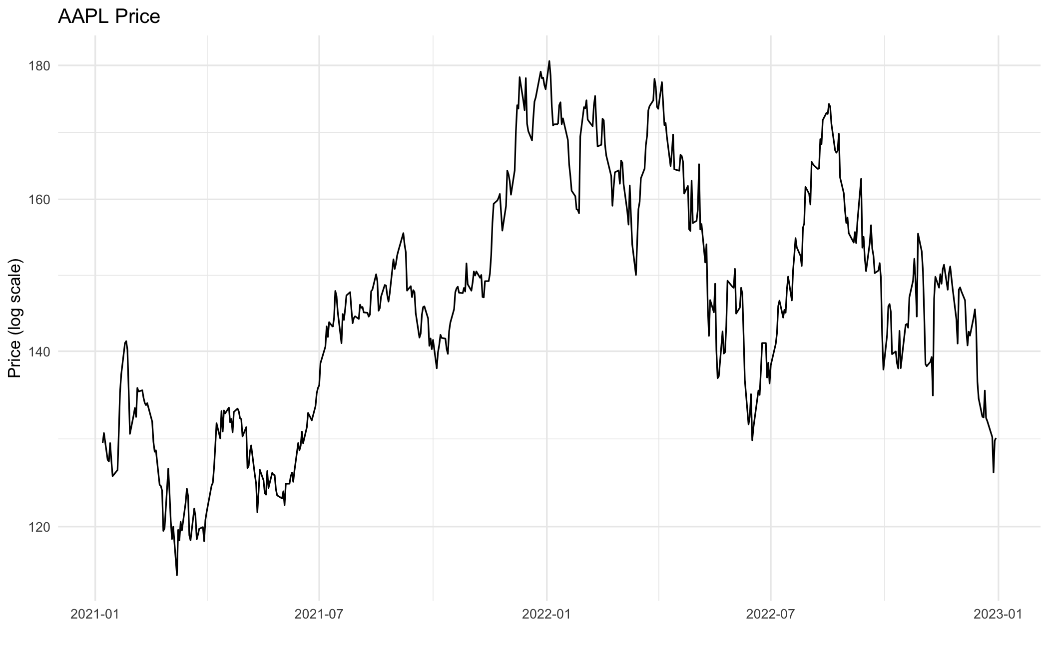
Chapter 12 covers plotting fundamentals. Here we embed plots in reports. Plots are embedded directly in the output when placed in code chunks:
```{r}
df_plot = data.frame(date = ymd(Prices$date), price = Prices$AAPL)
ggplot(df_plot, aes(x = date, y = price)) +
  geom_line() +
  scale_y_log10() +
  labs(title = "AAPL Price", x = "", y = "Price (log scale)") +
  theme_minimal()
```
This renders as:
```{python}
df_plot = pd.DataFrame({
    'date': Prices['date'],
    'price': Prices['AAPL']
})

(ggplot(df_plot, aes(x='date', y='price'))
 + geom_line()
 + scale_y_log10()
 + labs(title="AAPL Price", x="", y="Price (log scale)")
 + theme_minimal())
```
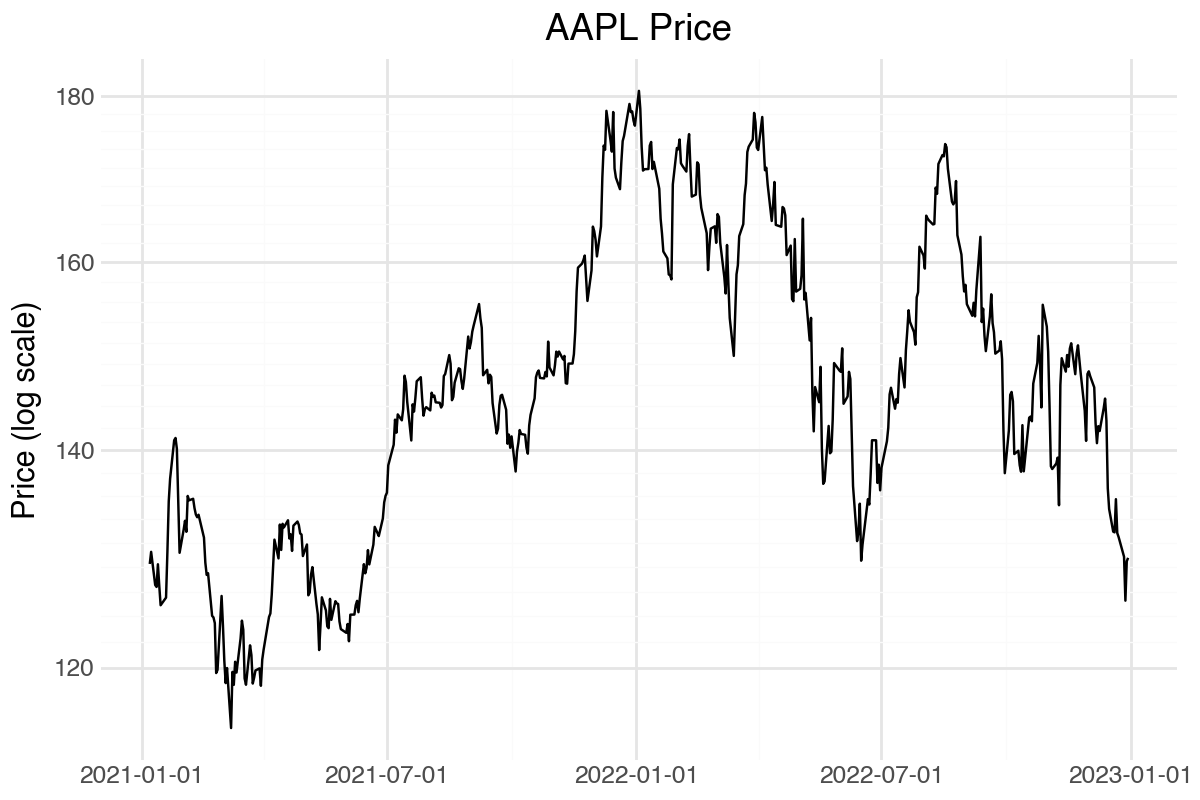
This renders as:
```{julia}
df_plot = DataFrame(
    date = Prices[!, "date"],
    price = Prices[!, "AAPL"]
);

p = ggplot(df_plot, @aes(x = date, y = price)) +
    geom_line() +
    scale_y_log10() +
    labs(title = "AAPL Price", x = "", y = "Price (log scale)") +
    theme_minimal()
```
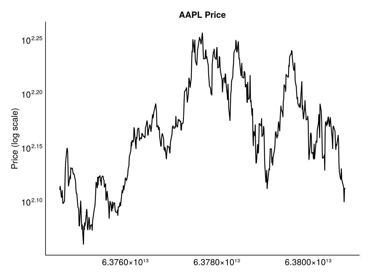
This renders as:
17.6 Creating tables
17.6.1 Basic text output
For multiple assets, we can create summary statistics programmatically:
```{r}
for(i in tickers){
  x = Returns[[i]]
  cat(sprintf("%s %.6f %.6f %.6f %.6f\n", i, mean(x), sd(x), min(x), max(x)))
}
```
This renders as:
AAPL 0.000076 0.019382 -0.060472 0.085236
DIS -0.001447 0.020029 -0.141139 0.061060
GE -0.000148 0.021152 -0.109101 0.068496
INTC -0.001189 0.022253 -0.124186 0.101278
JPM 0.000136 0.016246 -0.063434 0.060033
MCD 0.000534 0.011124 -0.049908 0.040062
```{python}
for ticker in tickers:
x = Returns[ticker]
print(f"{ticker} {x.mean():.6f} {x.std():.6f} {x.min():.6f} {x.max():.6f}")
```This renders as:
AAPL 0.000076 0.019382 -0.060472 0.085236
DIS -0.001447 0.020029 -0.141139 0.061060
GE -0.000148 0.021152 -0.109101 0.068496
INTC -0.001189 0.022253 -0.124186 0.101278
JPM 0.000136 0.016246 -0.063434 0.060033
MCD 0.000534 0.011124 -0.049908 0.040062
```{julia}
using Printf
for ticker in tickers
x = Returns[!, ticker]
@printf("%s %.6f %.6f %.6f %.6f\n", ticker, mean(x), std(x), minimum(x), maximum(x))
end
```This renders as:
AAPL 0.000076 0.019382 -0.060472 0.085236
DIS -0.001447 0.020029 -0.141139 0.061060
GE -0.000148 0.021152 -0.109101 0.068496
INTC -0.001189 0.022253 -0.124186 0.101278
JPM 0.000136 0.016246 -0.063434 0.060033
MCD 0.000534 0.011124 -0.049908 0.040062
17.6.2 Formatted tables
For better formatting, each language has table-rendering functions:
```{r}
library(knitr)

df = matrix(ncol = 5, nrow = length(tickers))
for(i in 1:length(tickers)){
  x = Returns[[tickers[i]]]
  lb = Box.test(x^2, lag = 10, type = "Ljung-Box")
  df[i,] = c(mean(x)*100, sd(x)*100, max(x)*100, lb$statistic, lb$p.value)
}

df = as.data.frame(df)
df = cbind(tickers, df)
names(df) = c("Asset", "Mean", "SD", "Max", "LB Stat", "LB p-val")

kable(df, digits = 3, caption = "Sample statistics")
```
This renders as:
Table: Sample statistics

|Asset |   Mean|    SD|    Max| LB Stat| LB p-val|
|:-----|------:|-----:|------:|-------:|--------:|
|AAPL  |  0.008| 1.938|  8.524|  55.333|    0.000|
|DIS   | -0.145| 2.003|  6.106|  13.945|    0.176|
|GE    | -0.015| 2.115|  6.850|  16.577|    0.084|
|INTC  | -0.119| 2.225| 10.128|   8.740|    0.557|
|JPM   |  0.014| 1.625|  6.003|  23.351|    0.010|
|MCD   |  0.053| 1.112|  4.006|  18.309|    0.050|
```{python}
#| output: asis
stats_data = []
for ticker in tickers:
x = Returns[ticker]
lb = acorr_ljungbox(x**2, lags=[10], return_df=True)
stats_data.append({
'Asset': ticker,
'Mean': round(x.mean() * 100, 3),
'SD': round(x.std() * 100, 3),
'Max': round(x.max() * 100, 3),
'LB Stat': round(lb['lb_stat'].values[0], 3),
'LB p-val': round(lb['lb_pvalue'].values[0], 3)
})
df_stats = pd.DataFrame(stats_data)
print(df_stats.to_html(index=False))
```This renders as:
<table border="1" class="dataframe">
  <thead>
    <tr style="text-align: right;">
      <th>Asset</th>
      <th>Mean</th>
      <th>SD</th>
      <th>Max</th>
      <th>LB Stat</th>
      <th>LB p-val</th>
    </tr>
  </thead>
  <tbody>
    <tr>
      <td>AAPL</td>
      <td>0.008</td>
      <td>1.938</td>
      <td>8.524</td>
      <td>55.333</td>
      <td>0.000</td>
    </tr>
    <tr>
      <td>DIS</td>
      <td>-0.145</td>
      <td>2.003</td>
      <td>6.106</td>
      <td>13.945</td>
      <td>0.176</td>
    </tr>
    <tr>
      <td>GE</td>
      <td>-0.015</td>
      <td>2.115</td>
      <td>6.850</td>
      <td>16.577</td>
      <td>0.084</td>
    </tr>
    <tr>
      <td>INTC</td>
      <td>-0.119</td>
      <td>2.225</td>
      <td>10.128</td>
      <td>8.740</td>
      <td>0.557</td>
    </tr>
    <tr>
      <td>JPM</td>
      <td>0.014</td>
      <td>1.625</td>
      <td>6.003</td>
      <td>23.351</td>
      <td>0.010</td>
    </tr>
    <tr>
      <td>MCD</td>
      <td>0.053</td>
      <td>1.112</td>
      <td>4.006</td>
      <td>18.309</td>
      <td>0.050</td>
    </tr>
  </tbody>
</table>
```{julia}
#| output: asis
function lb_test(x)
lb = LjungBoxTest(x.^2, 10)
return (lb.Q, pvalue(lb))
end
df_stats = DataFrame(
"Asset" => tickers,
"Mean" => [round(mean(Returns[!, t]) * 100, digits=3) for t in tickers],
"SD" => [round(std(Returns[!, t]) * 100, digits=3) for t in tickers],
"Max" => [round(maximum(Returns[!, t]) * 100, digits=3) for t in tickers],
"LB Stat" => [round(lb_test(Returns[!, t])[1], digits=3) for t in tickers],
"LB p-val" => [round(lb_test(Returns[!, t])[2], digits=3) for t in tickers]
)
io = IOBuffer()
pretty_table(io, df_stats, backend = :html)
print(String(take!(io)))
```This renders as:
<table>
  <thead>
    <tr class = "columnLabelRow">
      <th style = "font-weight: bold; text-align: right;">Asset</th>
      <th style = "font-weight: bold; text-align: right;">Mean</th>
      <th style = "font-weight: bold; text-align: right;">SD</th>
      <th style = "font-weight: bold; text-align: right;">Max</th>
      <th style = "font-weight: bold; text-align: right;">LB Stat</th>
      <th style = "font-weight: bold; text-align: right;">LB p-val</th>
    </tr>
    <tr class = "columnLabelRow">
      <th style = "text-align: right;">String</th>
      <th style = "text-align: right;">Float64</th>
      <th style = "text-align: right;">Float64</th>
      <th style = "text-align: right;">Float64</th>
      <th style = "text-align: right;">Float64</th>
      <th style = "text-align: right;">Float64</th>
    </tr>
  </thead>
  <tbody>
    <tr class = "dataRow">
      <td style = "text-align: right;">AAPL</td>
      <td style = "text-align: right;">0.008</td>
      <td style = "text-align: right;">1.938</td>
      <td style = "text-align: right;">8.524</td>
      <td style = "text-align: right;">55.333</td>
      <td style = "text-align: right;">0.0</td>
    </tr>
    <tr class = "dataRow">
      <td style = "text-align: right;">DIS</td>
      <td style = "text-align: right;">-0.145</td>
      <td style = "text-align: right;">2.003</td>
      <td style = "text-align: right;">6.106</td>
      <td style = "text-align: right;">13.945</td>
      <td style = "text-align: right;">0.176</td>
    </tr>
    <tr class = "dataRow">
      <td style = "text-align: right;">GE</td>
      <td style = "text-align: right;">-0.015</td>
      <td style = "text-align: right;">2.115</td>
      <td style = "text-align: right;">6.85</td>
      <td style = "text-align: right;">16.577</td>
      <td style = "text-align: right;">0.084</td>
    </tr>
    <tr class = "dataRow">
      <td style = "text-align: right;">INTC</td>
      <td style = "text-align: right;">-0.119</td>
      <td style = "text-align: right;">2.225</td>
      <td style = "text-align: right;">10.128</td>
      <td style = "text-align: right;">8.74</td>
      <td style = "text-align: right;">0.557</td>
    </tr>
    <tr class = "dataRow">
      <td style = "text-align: right;">JPM</td>
      <td style = "text-align: right;">0.014</td>
      <td style = "text-align: right;">1.625</td>
      <td style = "text-align: right;">6.003</td>
      <td style = "text-align: right;">23.351</td>
      <td style = "text-align: right;">0.01</td>
    </tr>
    <tr class = "dataRow">
      <td style = "text-align: right;">MCD</td>
      <td style = "text-align: right;">0.053</td>
      <td style = "text-align: right;">1.112</td>
      <td style = "text-align: right;">4.006</td>
      <td style = "text-align: right;">18.309</td>
      <td style = "text-align: right;">0.05</td>
    </tr>
  </tbody>
</table>
17.7 Inline code in reports
Inline code embeds calculated values directly in your prose. Rather than hardcoding numbers that might change, you reference variables or expressions that are evaluated when the document renders. This keeps your text synchronised with your analysis — if the data changes, the numbers in your text update automatically.
The syntax places the expression inside backticks with a language identifier. When Quarto renders the document, it evaluates the expression and substitutes the result. You can use simple variables or more complex expressions including calculations and function calls.
The knitr engine used throughout this book evaluates inline r expressions, but not inline python or julia expressions. Where the sections below show Python or Julia results, the rendered-looking sentence is static text illustrating what a native Quarto document would produce with the current data, not a live evaluation.
Suppose we want to report on r use stock. We write:
If we take `r use`, we have `r length(Returns[[use]])` observations. The mean return is `r round(mean(Returns[[use]])*100, 4)`%, and on the best day the return was `r round(max(Returns[[use]])*100, 1)`%.
If we take r use, we have r length(Returns[[use]]) observations. The mean return is r round(mean(Returns[[use]])*100, 4)%, and on the best day the return was r round(max(Returns[[use]])*100, 1)%.
If we take `{python} use`, we have `{python} len(Returns[use])` observations. The mean return is `{python} round(Returns[use].mean()*100, 4)`%, and on the best day the return was `{python} round(Returns[use].max()*100, 1)`%.
If we take AAPL, we have 500 observations. The mean return is 0.0076%, and on the best day the return was 8.5%.
If we take `{julia} use`, we have `{julia} length(Returns[!, use])` observations. The mean return is `{julia} round(mean(Returns[!, use])*100, digits=4)`%, and on the best day the return was `{julia} round(maximum(Returns[!, use])*100, digits=1)`%.
If we take AAPL, we have 500 observations. The mean return is 0.0076%, and on the best day the return was 8.5%.
17.7.1 Finding specific dates
We can find the dates of specific events like the best and worst returns. First we compute the dates in a code chunk:
```{r}
best_date = format(
  ymd(Returns$date[which.max(Returns[[use]])]),
  "%d %B %Y"
)
worst_date = format(
  ymd(Returns$date[which.min(Returns[[use]])]),
  "%d %B %Y"
)
```
The best day happened on `r best_date`. The worst day happened on `r worst_date`.
The best day happened on r best_date. The worst day happened on r worst_date.
```{python}
best_idx = Returns[use].idxmax()
worst_idx = Returns[use].idxmin()
best_date = Returns.loc[best_idx, 'date'].strftime("%d %B %Y")
worst_date = Returns.loc[worst_idx, 'date'].strftime("%d %B %Y")
```
The best day happened on `{python} best_date`. The worst day happened on `{python} worst_date`.
The best day happened on 10 November 2022. The worst day happened on 13 September 2022.
```{julia}
best_idx = argmax(Returns[!, use])
worst_idx = argmin(Returns[!, use])
best_date = Dates.format(Returns[best_idx, :date], "dd U Y")
worst_date = Dates.format(Returns[worst_idx, :date], "dd U Y")
```
The best day happened on `{julia} best_date`. The worst day happened on `{julia} worst_date`.
The best day happened on 10 November 2022. The worst day happened on 13 September 2022.
17.7.2 Statistical tests
Chapter 14 covers statistical test details. This section shows how to embed those results in prose. First compute the test in a hidden code chunk, then reference the results inline.
The GE returns have mean `r round(mean(y_r)*100, 4)`% and standard deviation `r round(sd(y_r)*100, 2)`%. The skewness is `r round(moments::skewness(y_r), 2)` and excess kurtosis is `r round(moments::kurtosis(y_r)-3, 2)`. The Jarque-Bera test has p-value `r format(jb\(p.value, digits=2)`</code>, rejecting normality. The Ljung-Box test on returns has p-value <code>`r round(lb_ret\)p.value, 3)`, while on squared returns the p-value is `r round(lb_sq$p.value, 3)`.
The GE returns have mean r round(mean(y_r)*100, 4)% and standard deviation r round(sd(y_r)*100, 2)%. The skewness is r round(moments::skewness(y_r), 2) and excess kurtosis is r round(moments::kurtosis(y_r)-3, 2). The Jarque-Bera test has p-value r format(jb$p.value, digits=2), rejecting normality. The Ljung-Box test on returns has p-value r round(lb_ret$p.value, 3), while on squared returns the p-value is r round(lb_sq$p.value, 3).
The GE returns have mean `{python} round(y_py.mean()*100, 4)`% and standard deviation `{python} round(y_py.std(ddof=1)*100, 2)`%. The skewness is `{python} round(skew(y_py), 2)` and excess kurtosis is `{python} round(kurtosis(y_py), 2)`. The Jarque-Bera test has p-value `{python} f”{jb_pval:.1e}“`, rejecting normality. The Ljung-Box test on returns has p-value `{python} round(lb_ret[‘lb_pvalue’].values[0], 3)`, while on squared returns the p-value is `{python} round(lb_sq[‘lb_pvalue’].values[0], 3)`.
The GE returns have mean -0.0148% and standard deviation 2.12%. The skewness is -0.37 and excess kurtosis is 1.89. The Jarque-Bera test has p-value 2.9e-19, rejecting normality. The Ljung-Box test on returns has p-value 0.309, while on squared returns the p-value is 0.084.
The GE returns have mean `{julia} round(mean(y_jl)*100, digits=4)`% and standard deviation `{julia} round(std(y_jl)*100, digits=2)`%. The skewness is `{julia} round(skewness(y_jl), digits=2)` and excess kurtosis is `{julia} round(kurtosis(y_jl), digits=2)`. The Jarque-Bera test has p-value `{julia} round(pvalue(jb), sigdigits=2)`, rejecting normality. The Ljung-Box test on returns has p-value `{julia} round(pvalue(lb_ret), digits=3)`, while on squared returns the p-value is `{julia} round(pvalue(lb_sq), digits=3)`.
The GE returns have mean -0.0148% and standard deviation 2.12%. The skewness is -0.37 and excess kurtosis is 1.89. The Jarque-Bera test has p-value 2.9e-19, rejecting normality. The Ljung-Box test on returns has p-value 0.309, while on squared returns the p-value is 0.084.
The pieces are now in place — a YAML header, code chunks, controlled display, embedded plots and tables, and inline values. Chapter 31 assembles them into three complete files, one per language, that you can copy and adapt.
Update the saved data and rerun the render, and everything in the document moves with it. That is the whole argument for writing reports this way.