library(ggplot2)
library(MASS)
library(copula)15 Simulations
We use simulations for three reasons. They test models, they show how models behave and they replace awkward mathematics with a numerical answer. Advanced applications of simulations in risk management, including Value-at-Risk calculations, are covered in Chapter 25.
When referring to simulations, we often use the term Monte Carlo after the Monte Carlo district of Monaco, a statelet on the Mediterranean coast surrounded by France and famous for its casino. We will use the terms simulation, Monte Carlo and MC interchangeably.
When doing simulations, we ask a computer algorithm to replicate the real world. But simulations have hard limits.
The first limit is simple. Computers are deterministic, so they do not produce true randomness. Instead, they produce something called a pseudorandom number, using an algorithm called a pseudorandom number generator. That is clumsy, so from here on we use the term random number generator or RNG.
A random number generator creates a sequence of numbers \(\UniformDraw_1, \UniformDraw_2, \ldots\) and when it has gone through the sequence, it starts again from the beginning. Therefore, if we know the internal state of the generator, we also know every subsequent draw \(\UniformDraw_{i+1}, \UniformDraw_{i+2}, \ldots\) in the sequence.
NoteThe same property outside finance
In cryptography, if attackers can determine the internal state of an RNG used for key generation, they may be able to predict future keys and compromise security. The predictability that makes simulation reproducible is exactly what makes a cipher breakable.
The second limit is that a simulation is a crude approximation of reality. If a model appears to pass or fail inside the simulation, that verdict need not survive contact with the market.
The length of the sequence before the RNG repeats is known as the period. The default random number generators in R and in Python’s random module use the Mersenne Twister algorithm, with a period of \(2^{19937}-1\), approximately \(10^{6002}\). NumPy’s legacy interface, np.random, used throughout this chapter, also employs the Mersenne Twister, while NumPy’s newer default_rng() interface uses PCG64 instead. Julia uses Xoshiro256++, with a period of \(2^{256}-1\). All are more than sufficient for almost every possible application.
The term seed refers to a particular starting point in the sequence of random numbers. The commands for setting the seed are set.seed() in R, np.random.seed() in Python and Random.seed!() in Julia. If one sets the seed to 1, one always gets the same random numbers. Setting the seed to 2 does not start the sequence at its second element. It starts from a different point on the loop altogether.
15.1 Data and libraries
Simulation needs a random number generator, which is built in, and a copula package, which is not.
import numpy as np
import pandas as pd
from scipy import stats
from scipy.stats import norm
from plotnine import ggplot, aes, geom_line, geom_point, geom_histogram, geom_vline
from plotnine import labs, theme, theme_minimal, annotate, coord_cartesian
import os

os.makedirs("_figs", exist_ok=True)
using Random, Statistics, Distributions, DataFrames
using TidierPlots, CairoMakie
using Copulas
isdir("_figs") || mkdir("_figs");15.2 Random numbers
15.2.1 Basics
In Section 14.3, we discussed the various distributions built into each language. To obtain simulated random numbers from a standard normal distribution:
rnorm(n = 1)
rnorm(n = 5)
[1] 0.3724005
[1] 0.29848646 -0.85994134 -0.55162714 -0.01996858 -0.82093295Every time we call the function, we get a different random number:
rnorm(n = 1)
rnorm(n = 1)
[1] 0.2400226
[1] 0.1131np.random.normal()
np.random.normal(size=5)Every time we call the function, we get a different random number:
print(np.random.normal())
print(np.random.normal())
-1.5928895261117963
0.5499585872184823randn()
randn(5)Every time we call the function, we get a different random number:
println(randn())
println(randn())
-0.27752111502844873
-0.938884310063784615.2.2 Seed
Most of the time we want the same random numbers each time we run an algorithm.
Since random number generators create a sequence of numbers that repeats, if we fix a place in the sequence, we always get the same random numbers. The way to do that is to set the seed.
rnorm(3)
rnorm(3)
set.seed(666)
rnorm(3)
set.seed(666)
rnorm(3)
[1] 0.5757169 -0.4072666 -0.9656123
[1] 0.5719939 -1.8196830 0.2065523
[1] 0.7533110 2.0143547 -0.3551345
[1] 0.7533110 2.0143547 -0.3551345print(np.random.normal(size=3))
print(np.random.normal(size=3))
np.random.seed(666)
print(np.random.normal(size=3))
np.random.seed(666)
print(np.random.normal(size=3))[-0.67446082 -0.39638296 -0.67915395]
[-2.47768163 -0.33524818 -0.89908978]
[0.82418808 0.479966 1.17346801]
[0.82418808 0.479966 1.17346801]println(randn(3))
println(randn(3))
Random.seed!(666);
println(randn(3))
Random.seed!(666);
println(randn(3))[1.3085509795079397, -0.6031101292935653, 0.3664946998032432]
[0.054970529246164, 1.7418421289806596, 0.7044954116027843]
[-1.0755336429985016, -0.4358053366724109, -0.7459634539487185]
[-1.0755336429985016, -0.4358053366724109, -0.7459634539487185]15.3 Distributions
We use four distributions for simulation — normal, Student-t, chi-square and Bernoulli. See Section 14.3 for distribution functions (PDF, CDF, quantile). Here we focus on random number generation.
cat("Normal:", round(rnorm(n = 1), 4), "\n")
cat("Student-t:", round(rt(n = 1, df = 3), 4), "\n")
cat("Chi-square:", round(rchisq(n = 1, df = 2), 4), "\n")
cat("Bernoulli:", rbinom(n = 1, size = 1, prob = 0.5), "\n")
Normal: 2.0282
Student-t: -1.9686
Chi-square: 4.3524
Bernoulli: 1print(f"Normal: {np.random.normal():.4f}")
print(f"Student-t: {np.random.standard_t(df=3):.4f}")
print(f"Chi-square: {np.random.chisquare(df=2):.4f}")
print(f"Bernoulli: {np.random.binomial(n=1, p=0.5)}")Normal: 0.9090
Student-t: -0.6826
Chi-square: 1.4188
Bernoulli: 0println("Normal: ", round(rand(Normal()), digits=4))
println("Student-t: ", round(rand(TDist(3)), digits=4))
println("Chi-square: ", round(rand(Chisq(2)), digits=4))
println("Bernoulli: ", rand(Binomial(1, 0.5)))Normal: -0.0324
Student-t: -4.8805
Chi-square: 0.5503
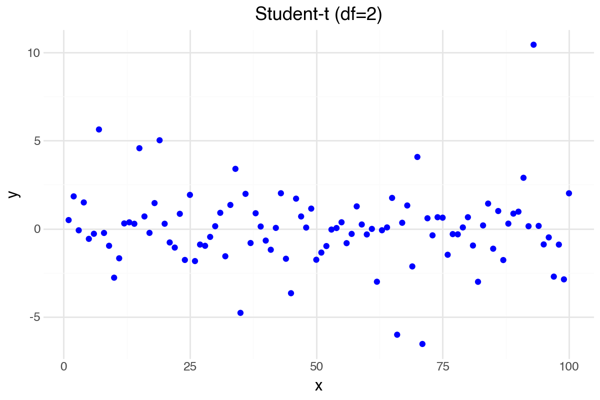
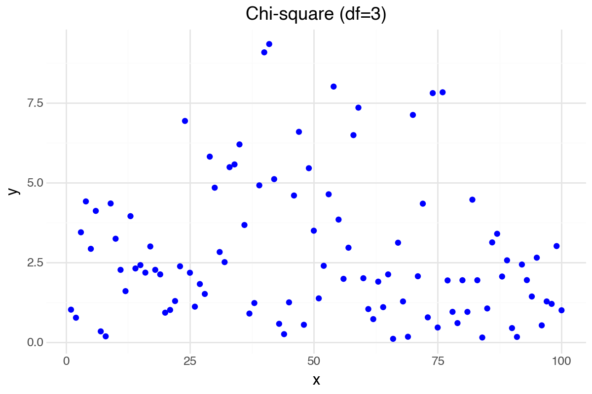
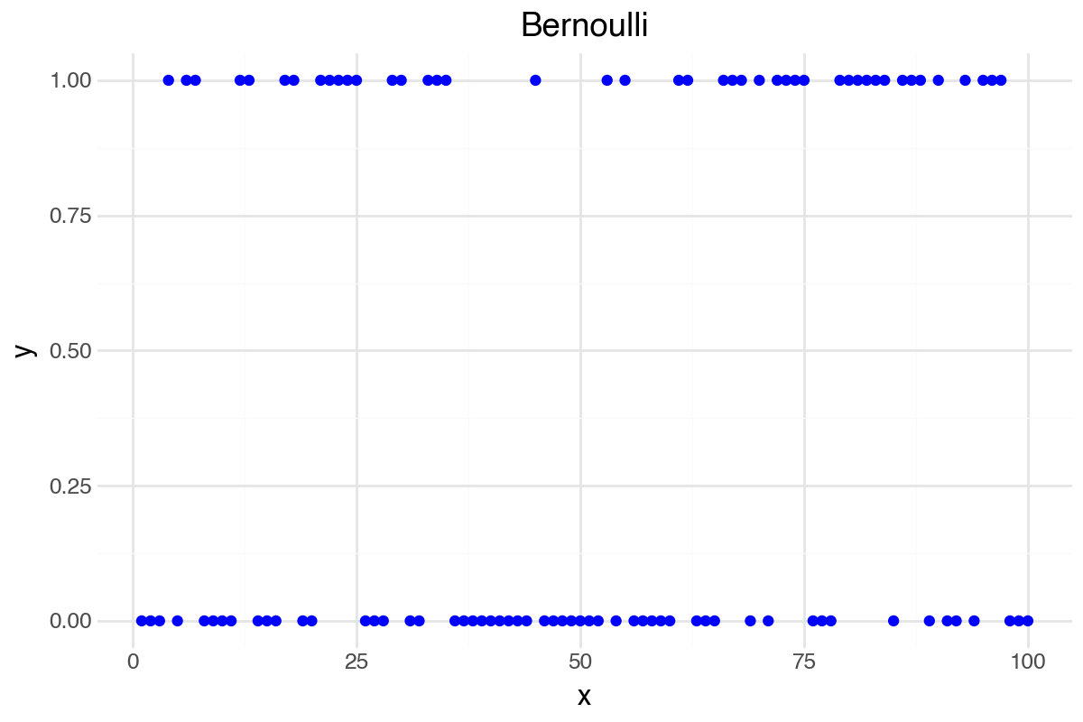
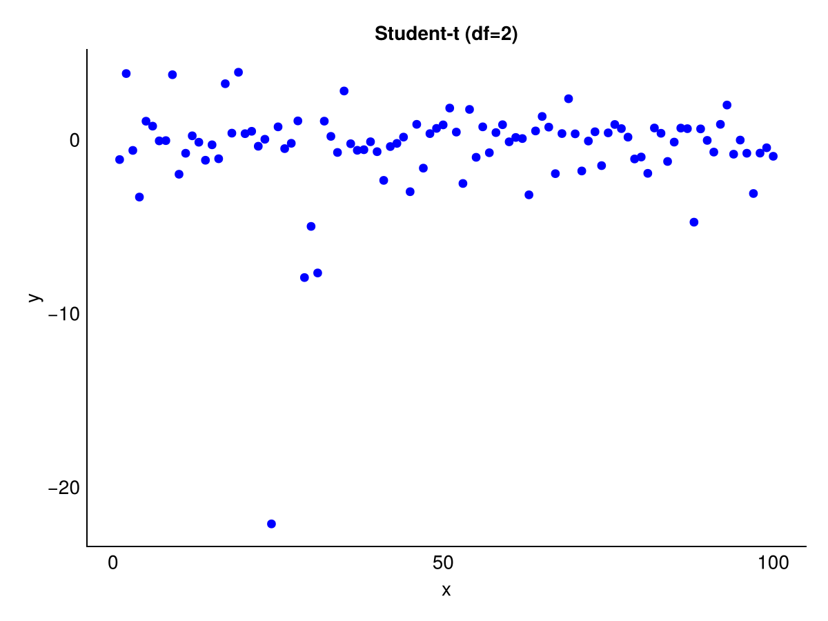
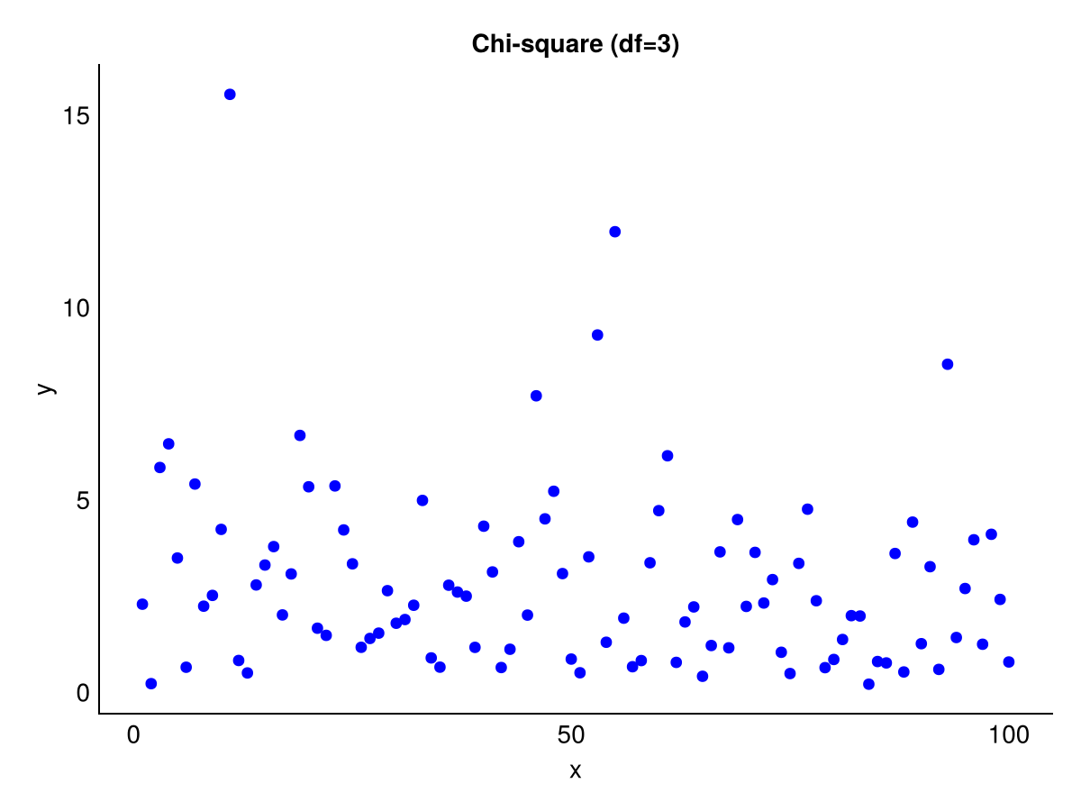
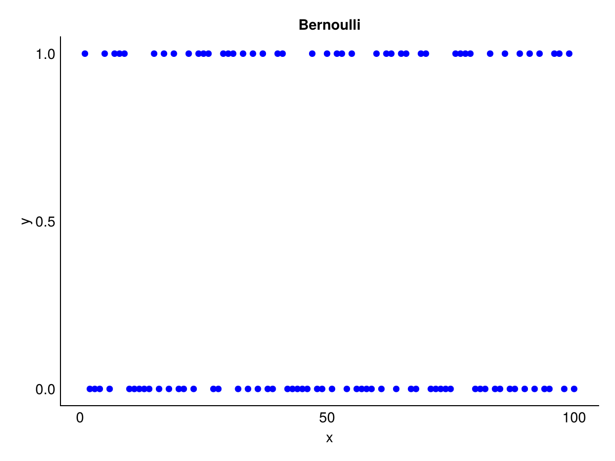
Bernoulli: 1We can also plot some random numbers.
df_norm = data.frame(x = 1:100, y = rnorm(n = 100))
ggplot(df_norm, aes(x = x, y = y)) +
  geom_point(colour = "blue") +
  labs(title = "Normal") +
  theme_minimal()

df_t = data.frame(x = 1:100, y = rt(n = 100, df = 2))
ggplot(df_t, aes(x = x, y = y)) +
  geom_point(colour = "blue") +
  labs(title = "Student-t (df=2)") +
  theme_minimal()

df_chi = data.frame(x = 1:100, y = rchisq(n = 100, df = 3))
ggplot(df_chi, aes(x = x, y = y)) +
  geom_point(colour = "blue") +
  labs(title = "Chi-square (df=3)") +
  theme_minimal()

df_binom = data.frame(x = 1:100, y = rbinom(n = 100, size = 1, prob = 0.5))
ggplot(df_binom, aes(x = x, y = y)) +
  geom_point(colour = "blue") +
  labs(title = "Bernoulli") +
  theme_minimal()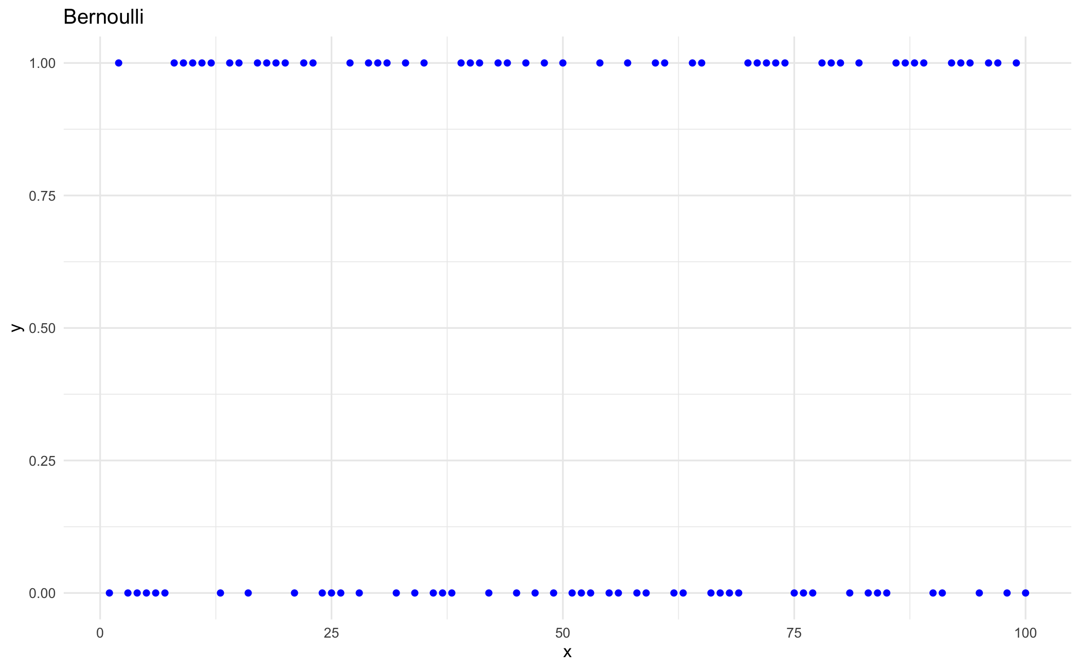
df_norm = pd.DataFrame({'x': range(1, 101), 'y': np.random.normal(size=100)})
p = (ggplot(df_norm, aes(x='x', y='y'))
 + geom_point(colour="blue")
 + labs(title="Normal")
 + theme_minimal())
p.save("_figs/sim_norm_py.png", width=6, height=4, dpi=100, verbose=False)

df_t = pd.DataFrame({'x': range(1, 101), 'y': np.random.standard_t(df=2, size=100)})
p = (ggplot(df_t, aes(x='x', y='y'))
 + geom_point(colour="blue")
 + labs(title="Student-t (df=2)")
 + theme_minimal())
p.save("_figs/sim_t_py.png", width=6, height=4, dpi=100, verbose=False)

df_chi = pd.DataFrame({'x': range(1, 101), 'y': np.random.chisquare(df=3, size=100)})
p = (ggplot(df_chi, aes(x='x', y='y'))
 + geom_point(colour="blue")
 + labs(title="Chi-square (df=3)")
 + theme_minimal())
p.save("_figs/sim_chi_py.png", width=6, height=4, dpi=100, verbose=False)

df_binom = pd.DataFrame({'x': range(1, 101), 'y': np.random.binomial(n=1, p=0.5, size=100)})
p = (ggplot(df_binom, aes(x='x', y='y'))
 + geom_point(colour="blue")
 + labs(title="Bernoulli")
 + theme_minimal())
p.save("_figs/sim_binom_py.png", width=6, height=4, dpi=100, verbose=False)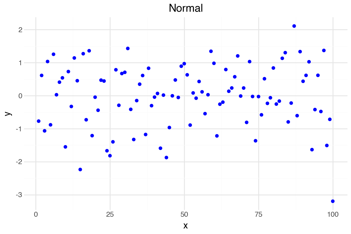
df_norm = DataFrame(x = 1:100, y = randn(100));
p = ggplot(df_norm, @aes(x = x, y = y)) +
    geom_point(color = "blue") +
    labs(title = "Normal") +
    theme_minimal();
ggsave("_figs/sim_norm_jl.png", p);

df_t = DataFrame(x = 1:100, y = rand(TDist(2), 100));
p = ggplot(df_t, @aes(x = x, y = y)) +
    geom_point(color = "blue") +
    labs(title = "Student-t (df=2)") +
    theme_minimal();
ggsave("_figs/sim_t_jl.png", p);

df_chi = DataFrame(x = 1:100, y = rand(Chisq(3), 100));
p = ggplot(df_chi, @aes(x = x, y = y)) +
    geom_point(color = "blue") +
    labs(title = "Chi-square (df=3)") +
    theme_minimal();
ggsave("_figs/sim_chi_jl.png", p);

df_binom = DataFrame(x = 1:100, y = rand(Binomial(1, 0.5), 100));
p = ggplot(df_binom, @aes(x = x, y = y)) +
    geom_point(color = "blue") +
    labs(title = "Bernoulli") +
    theme_minimal();
ggsave("_figs/sim_binom_jl.png", p);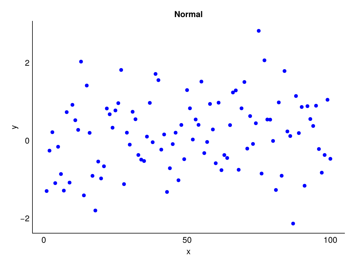
A combined plot reveals the distributions more clearly.
n = 100
df_all = data.frame(
  x = rep(1:n, 4),
  y = c(rnorm(n), rt(n, df = 3), rchisq(n, df = 2), rbinom(n, size = 1, prob = 0.5)),
  distribution = rep(c("Normal", "Student-t", "Chi-square", "Bernoulli"), each = n)
)

ggplot(df_all, aes(x = x, y = y, colour = distribution)) +
  geom_point() +
  labs(x = "", y = "", colour = NULL) +
  theme_minimal() +
  theme(legend.position = "top")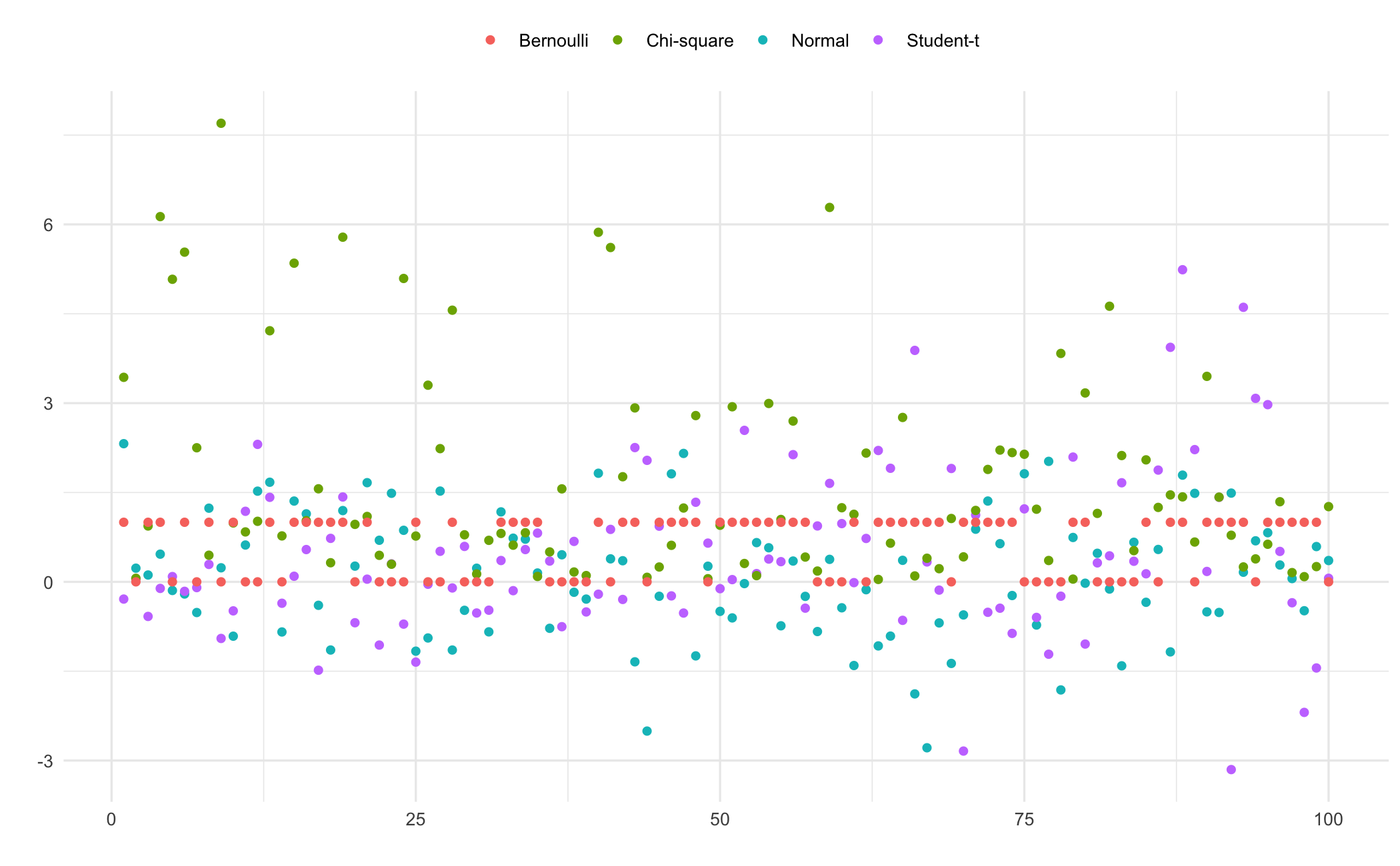
n = 100
df_all = pd.DataFrame({
    'x': list(range(1, n+1)) * 4,
    'y': np.concatenate([
        np.random.normal(size=n),
        np.random.standard_t(df=3, size=n),
        np.random.chisquare(df=2, size=n),
        np.random.binomial(n=1, p=0.5, size=n)
    ]),
    'distribution': ['Normal']*n + ['Student-t']*n + ['Chi-square']*n + ['Bernoulli']*n
})

p = (ggplot(df_all, aes(x='x', y='y', colour='distribution'))
 + geom_point()
 + labs(x="", y="", colour="")
 + theme_minimal()
 + theme(legend_position="top"))
p.save("_figs/sim_all_py.png", width=6, height=4, dpi=100, verbose=False)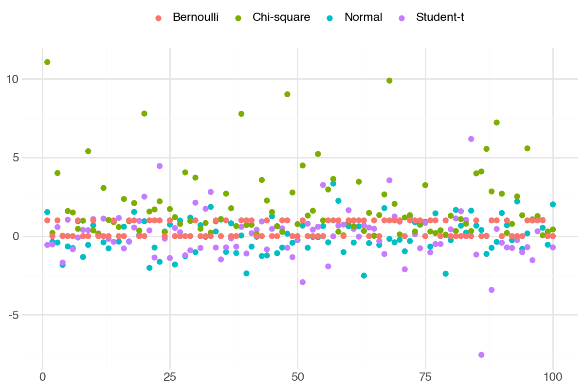
n = 100;
df_all = DataFrame(
    x = repeat(1:n, 4),
    y = vcat(randn(n), rand(TDist(3), n), rand(Chisq(2), n), rand(Binomial(1, 0.5), n)),
    distribution = vcat(fill("Normal", n), fill("Student-t", n), fill("Chi-square", n), fill("Bernoulli", n))
);

p = ggplot(df_all, @aes(x = x, y = y, color = distribution)) +
    geom_point() +
    labs(x = "", y = "") +
    theme_minimal();
ggsave("_figs/sim_all_jl.png", p);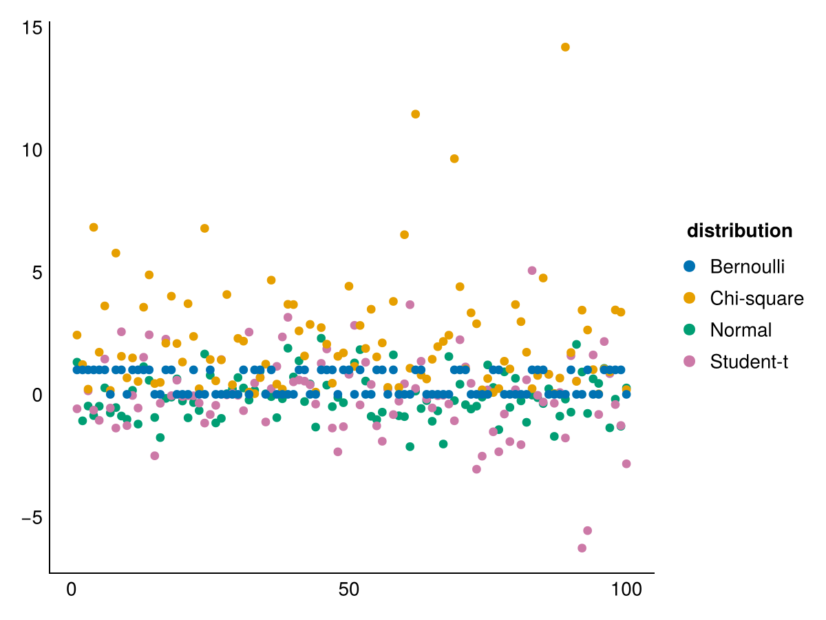
15.4 Number of simulations
A common problem in simulations is to determine the number of necessary simulations. Pick too few, and one gets an inaccurate simulation estimate. Pick too many, and one wastes resources.
By the Central Limit Theorem, the standard error of the Monte Carlo estimate decreases at rate \(O(1/\sqrt{\NumberSims})\), provided the simulated quantity has finite variance. The rate does not depend on the dimension of the problem, though the constant depends on the variance of the quantity being estimated. Here \(\NumberSims\) corresponds to S in the code below.
Below, we pick six simulation sizes and see how well their mean and standard deviation compare to the known true value (mean=1, sd=2).
S = c(5, 25, 100, 1e3, 1e4, 1e5)
results = data.frame(n = S, mean = NA, sd = NA)
for(i in seq_along(S)){
  x = rnorm(n = S[i], mean = 1, sd = 2)
  results$mean[i] = round(mean(x), 4)
  results$sd[i] = round(sd(x), 4)
}
results$meanError = round(results$mean - 1, 4)
results$sdError = round(results$sd - 2, 4)
print(results)
n mean sd meanError sdError
1 5 0.8619 1.8499 -0.1381 -0.1501
2 25 0.9884 2.1266 -0.0116 0.1266
3 100 1.1234 1.9187 0.1234 -0.0813
4 1000 0.9880 1.9825 -0.0120 -0.0175
5 10000 1.0000 2.0056 0.0000 0.0056
6 100000 1.0027 1.9973 0.0027 -0.0027S = [5, 25, 100, 1000, 10000, 100000]
results = []
for n in S:
x = np.random.normal(loc=1, scale=2, size=n)
results.append({'n': n, 'mean': round(np.mean(x), 4), 'sd': round(np.std(x, ddof=1), 4)})
df_results = pd.DataFrame(results)
df_results['meanError'] = round(df_results['mean'] - 1, 4)
df_results['sdError'] = round(df_results['sd'] - 2, 4)
print(df_results.to_string(index=False)) n mean sd meanError sdError
5 1.0602 0.8846 0.0602 -1.1154
25 1.3348 1.6687 0.3348 -0.3313
100 0.7176 1.9888 -0.2824 -0.0112
1000 1.0109 1.9673 0.0109 -0.0327
10000 1.0037 1.9889 0.0037 -0.0111
100000 1.0101 2.0000 0.0101 0.0000S = [5, 25, 100, 1000, 10000, 100000];
results = DataFrame(n = S, mean = zeros(length(S)), sd = zeros(length(S)));
for (i, n) in enumerate(S)
x = rand(Normal(1, 2), n);
results.mean[i] = round(mean(x), digits=4);
results.sd[i] = round(std(x), digits=4);
end
results.meanError = round.(results.mean .- 1, digits=4);
results.sdError = round.(results.sd .- 2, digits=4);
println(results)6×5 DataFrame
Row │ n mean sd meanError sdError
│ Int64 Float64 Float64 Float64 Float64
─────┼──────────────────────────────────────────────
1 │ 5 0.8817 2.498 -0.1183 0.498
2 │ 25 0.5555 2.1691 -0.4445 0.1691
3 │ 100 1.0394 2.0443 0.0394 0.0443
4 │ 1000 0.9102 1.9519 -0.0898 -0.0481
5 │ 10000 1.0147 1.9914 0.0147 -0.0086
6 │ 100000 1.0041 1.9905 0.0041 -0.009515.5 Random walk
It is easy to simulate a random walk. In the example below, we set the mean to 0 and the standard deviation to 1%, which is approximately correct for most stock returns. We also use the IID normal distribution, which is not correct for stock returns. A simple return below -100% would produce a negative price, but at this standard deviation that is a draw beyond 100 standard deviations and does not occur in practice. Simulating log returns and exponentiating, as the option-pricing section below does, avoids the bound entirely.
N = 1000
x = rnorm(N, mean = 0, sd = 0.01)
p = cumprod(c(1, x + 1))
df_rw = data.frame(t = 0:N, price = p)
ggplot(df_rw, aes(x = t, y = price)) +
  geom_line() +
  labs(x = "", y = "Price") +
  theme_minimal()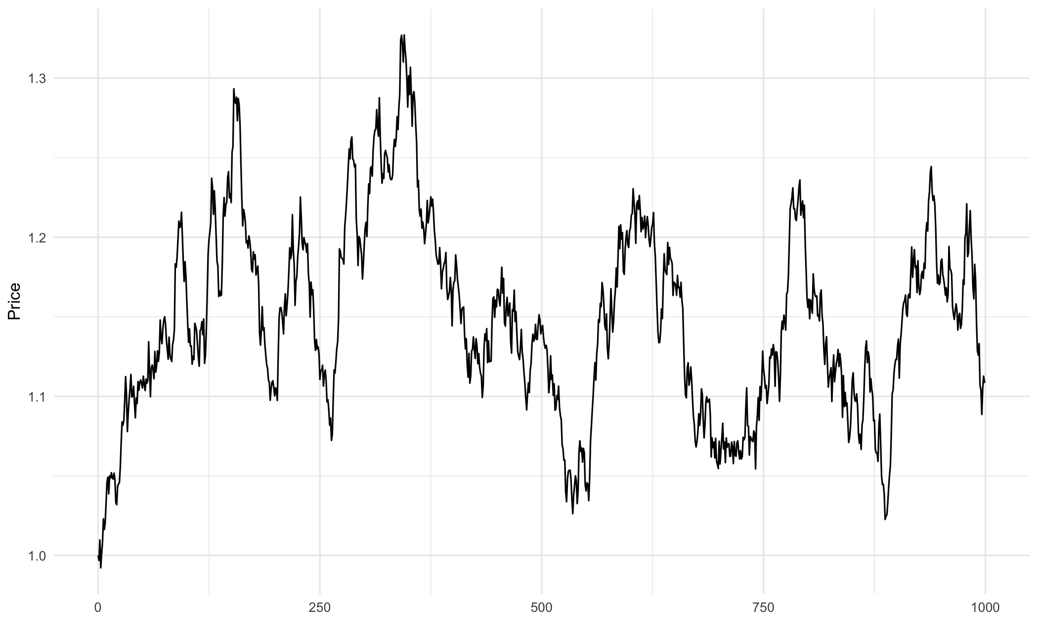
N = 1000
x = np.random.normal(loc=0, scale=0.01, size=N)
p = np.cumprod(np.concatenate(([1], x + 1)))
df_rw = pd.DataFrame({'t': range(0, N+1), 'price': p})

p_plot = (ggplot(df_rw, aes(x='t', y='price'))
 + geom_line()
 + labs(x="", y="Price")
 + theme_minimal())
p_plot.save("_figs/sim_rw_py.png", width=6, height=4, dpi=100, verbose=False)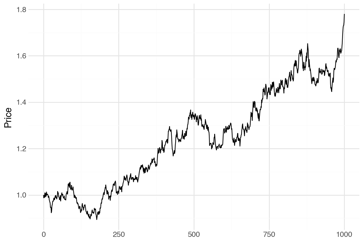
N = 1000;
x = randn(N) * 0.01;
p = cumprod(vcat(1, x .+ 1));
df_rw = DataFrame(t = 0:N, price = p);

pl = ggplot(df_rw, @aes(x = t, y = price)) +
    geom_line() +
    labs(x = "", y = "Price") +
    theme_minimal();
ggsave("_figs/sim_rw_jl.png", pl);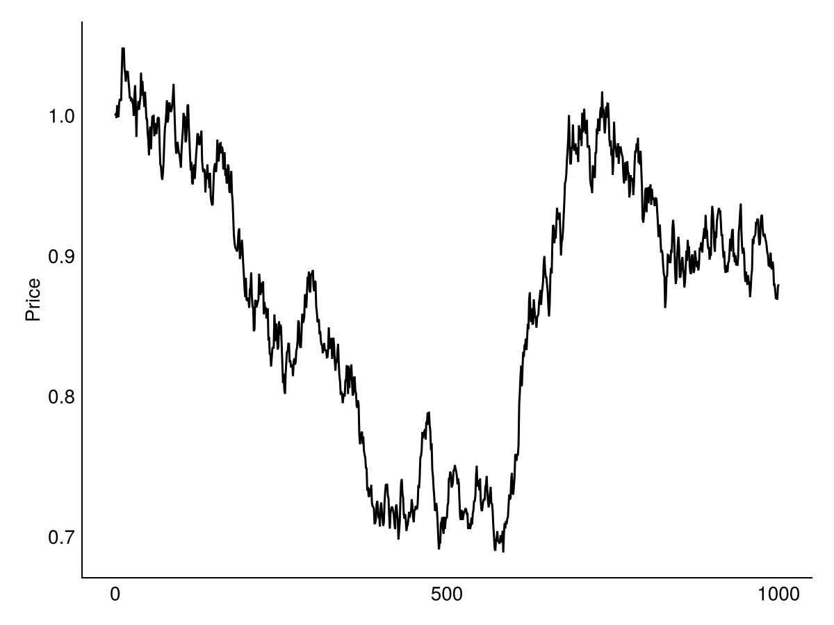
We can also do several random walks and plot them on the same figure.
N = 1000
R = 4
df_walks = do.call(rbind, lapply(1:R, function(i) {
  x = rnorm(N, mean = 0, sd = 0.01)
  p = cumprod(c(1, x + 1))
  data.frame(t = 0:N, price = p, walk = factor(i))
}))

ggplot(df_walks, aes(x = t, y = price, colour = walk)) +
  geom_line() +
  labs(x = "", y = "Price", colour = NULL) +
  theme_minimal()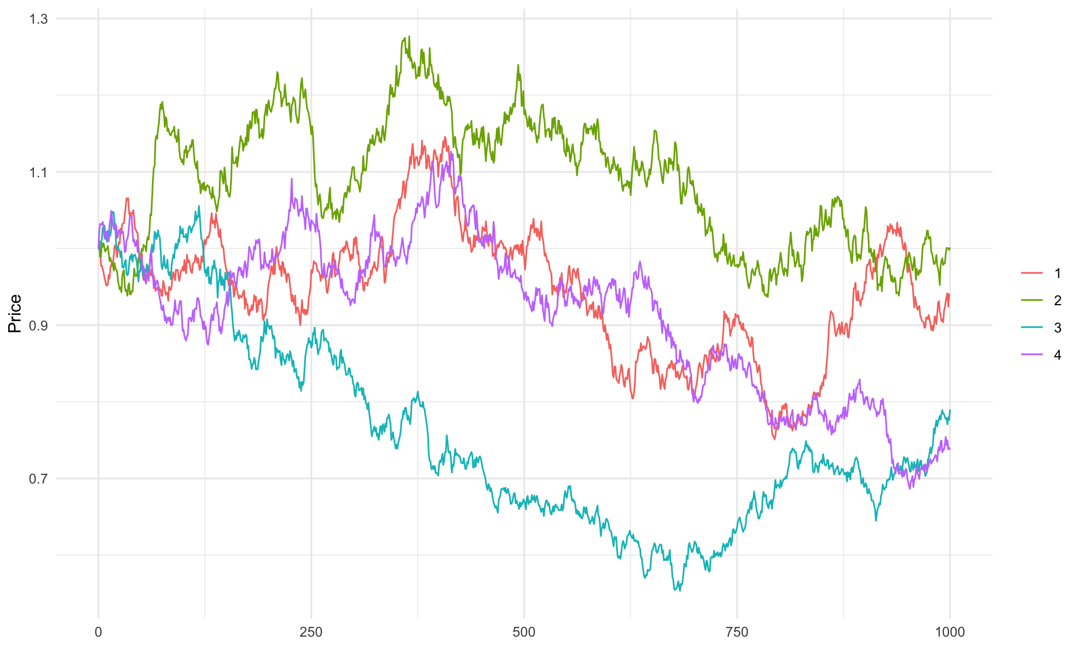
N = 1000
R = 4
walks = []
for i in range(R):
    x = np.random.normal(loc=0, scale=0.01, size=N)
    p = np.cumprod(np.concatenate(([1], x + 1)))
    walks.append(pd.DataFrame({'t': range(0, N+1), 'price': p, 'walk': str(i+1)}))
df_walks = pd.concat(walks)

p_plot = (ggplot(df_walks, aes(x='t', y='price', colour='walk'))
 + geom_line()
 + labs(x="", y="Price", colour="")
 + theme_minimal())
p_plot.save("_figs/sim_walks_py.png", width=6, height=4, dpi=100, verbose=False)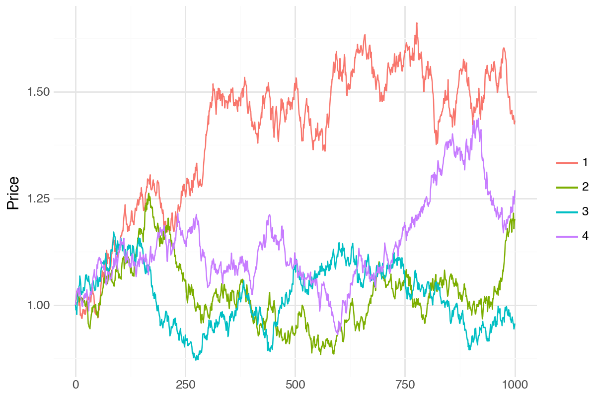
N = 1000;
R = 4;
df_walks = vcat([begin
    x = randn(N) * 0.01;
    p = cumprod(vcat(1, x .+ 1));
    DataFrame(t = 0:N, price = p, walk = fill(string(i), N+1))
end for i in 1:R]...);

pl = ggplot(df_walks, @aes(x = t, y = price, color = walk)) +
    geom_line() +
    labs(x = "", y = "Price") +
    theme_minimal();
ggsave("_figs/sim_walks_jl.png", pl);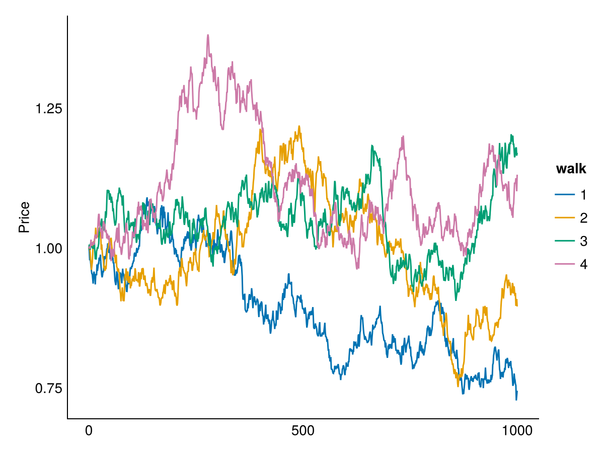
The random walk above simulates a price path by compounding IID returns. Option pricing extends this idea. Instead of tracing a path, we simulate the terminal asset price under a specific model, such as geometric Brownian motion, and compute the discounted payoff. By averaging over many such simulated payoffs, we obtain a Monte Carlo estimate of the option price.
15.6 Pricing options
This is the cleanest test of Monte Carlo pricing. Black-Scholes gives the exact option value, so any gap comes from simulation error.
Start with a function for the Black-Scholes price and set some parameters.
bs = function(X, P, r, sigma, T){
  d1 = (log(P/X) + (r + 0.5*sigma^2)*T) / (sigma*sqrt(T))
  d2 = d1 - sigma*sqrt(T)
  Call = P*pnorm(d1) - X*exp(-r*T)*pnorm(d2)
  Put = X*exp(-r*T)*pnorm(-d2) - P*pnorm(-d1)
  return(list(Call = Call, Put = Put))
}

P0 = 50; sigma = 0.2; r = 0.05; T = 0.5; X = 40
bsprice = bs(X, P0, r, sigma, T)
cat("Call:", round(bsprice$Call, 4), "\n")
cat("Put:", round(bsprice$Put, 4), "\n")
Call: 11.0873
Put: 0.0997def bs(X, P, r, sigma, T):
d1 = (np.log(P/X) + (r + 0.5*sigma**2)*T) / (sigma*np.sqrt(T))
d2 = d1 - sigma*np.sqrt(T)
Call = P*norm.cdf(d1) - X*np.exp(-r*T)*norm.cdf(d2)
Put = X*np.exp(-r*T)*norm.cdf(-d2) - P*norm.cdf(-d1)
return {'Call': Call, 'Put': Put}
P0 = 50; sigma = 0.2; r = 0.05; T = 0.5; X = 40
bsprice = bs(X, P0, r, sigma, T)
print(f"Call: {bsprice['Call']:.4f}")
print(f"Put: {bsprice['Put']:.4f}")Call: 11.0873
Put: 0.0997function bs(X, P, r, sigma, T)
d1 = (log(P/X) + (r + 0.5*sigma^2)*T) / (sigma*sqrt(T));
d2 = d1 - sigma*sqrt(T);
Call = P*cdf(Normal(), d1) - X*exp(-r*T)*cdf(Normal(), d2);
Put = X*exp(-r*T)*cdf(Normal(), -d2) - P*cdf(Normal(), -d1);
return (Call = Call, Put = Put)
end
P0 = 50; sigma = 0.2; r = 0.05; T = 0.5; X = 40;
bsprice = bs(X, P0, r, sigma, T);
println("Call: ", round(bsprice.Call, digits=4))
println("Put: ", round(bsprice.Put, digits=4))Call: 11.0873
Put: 0.0997We then create a simulation function that returns the discounted payoff draws for a call option, and test it.
sim = function(S = 1e6, P0 = 50, sigma = 0.2, r = 0.05, T = 0.5, X = 40, seed = 666){
  set.seed(seed)
  F = P0 * exp(r * T)
  ysim = rnorm(S, -0.5 * sigma^2 * T, sigma * sqrt(T))
  F = F * exp(ysim)
  SP = pmax(F - X, 0)
  fsim = SP * exp(-r * T)
  return(fsim)
}

cat("Mean:", round(mean(sim(S = 10)), 4), "\n")
Mean: 11.1472def sim(S=1000000, P0=50, sigma=0.2, r=0.05, T=0.5, X=40, seed=666):
np.random.seed(seed)
F = P0 * np.exp(r * T)
ysim = np.random.normal(-0.5 * sigma**2 * T, sigma * np.sqrt(T), S)
F = F * np.exp(ysim)
SP = np.maximum(F - X, 0)
fsim = SP * np.exp(-r * T)
return fsim
print(f"Mean: {np.mean(sim(S=10)):.4f}")Mean: 11.9051function sim(S=1000000; P0=50, sigma=0.2, r=0.05, T=0.5, X=40, seed=666)
Random.seed!(seed);
F = P0 * exp(r * T);
ysim = rand(Normal(-0.5 * sigma^2 * T, sigma * sqrt(T)), S);
F = F .* exp.(ysim);
SP = max.(F .- X, 0);
fsim = SP .* exp(-r * T);
return fsim
end
println("Mean: ", round(mean(sim(10)), digits=4))Mean: 12.2977If we let the number of simulations vary, we can see convergence to the true value:
cat(paste0("Black-Scholes: ", round(bsprice$Call, 4), "\n"))
for(S in c(10, 50, 100, 1000, 10000)){
  cat(paste0(S, ": ", round(mean(sim(S = S)), 4), "\n"))
}
Black-Scholes: 11.0873
10: 11.1472
50: 10.7544
100: 10.6525
1000: 10.9352
10000: 11.1966print(f"Black-Scholes: {bsprice['Call']:.4f}")
for S in [10, 50, 100, 1000, 10000]:
print(f"{S}: {np.mean(sim(S=S)):.4f}")Black-Scholes: 11.0873
10: 11.9051
50: 10.5451
100: 10.9802
1000: 11.0301
10000: 10.9720println("Black-Scholes: ", round(bsprice.Call, digits=4))
for S in [10, 50, 100, 1000, 10000]
println(S, ": ", round(mean(sim(S; seed=666)), digits=4))
endBlack-Scholes: 11.0873
10: 12.2977
50: 12.8988
100: 12.3689
1000: 11.3754
10000: 11.1202Below, we run many more simulations and plot their histogram with the true value superimposed.
fsim = sim()
df_hist = data.frame(price = fsim)

ggplot(df_hist, aes(x = price)) +
  geom_histogram(aes(y = after_stat(density)), breaks = seq(0, 35, length.out = 101), fill = "red", colour = "white") +
  geom_vline(xintercept = bsprice$Call, colour = "darkred", linewidth = 1) +
  annotate("text", x = bsprice$Call, y = 0.11, label = "Black-Scholes\ncall price", hjust = -0.1) +
  coord_cartesian(ylim = c(0, 0.12)) +
  labs(x = "Discounted call payoff draws", y = "Density") +
  theme_minimal()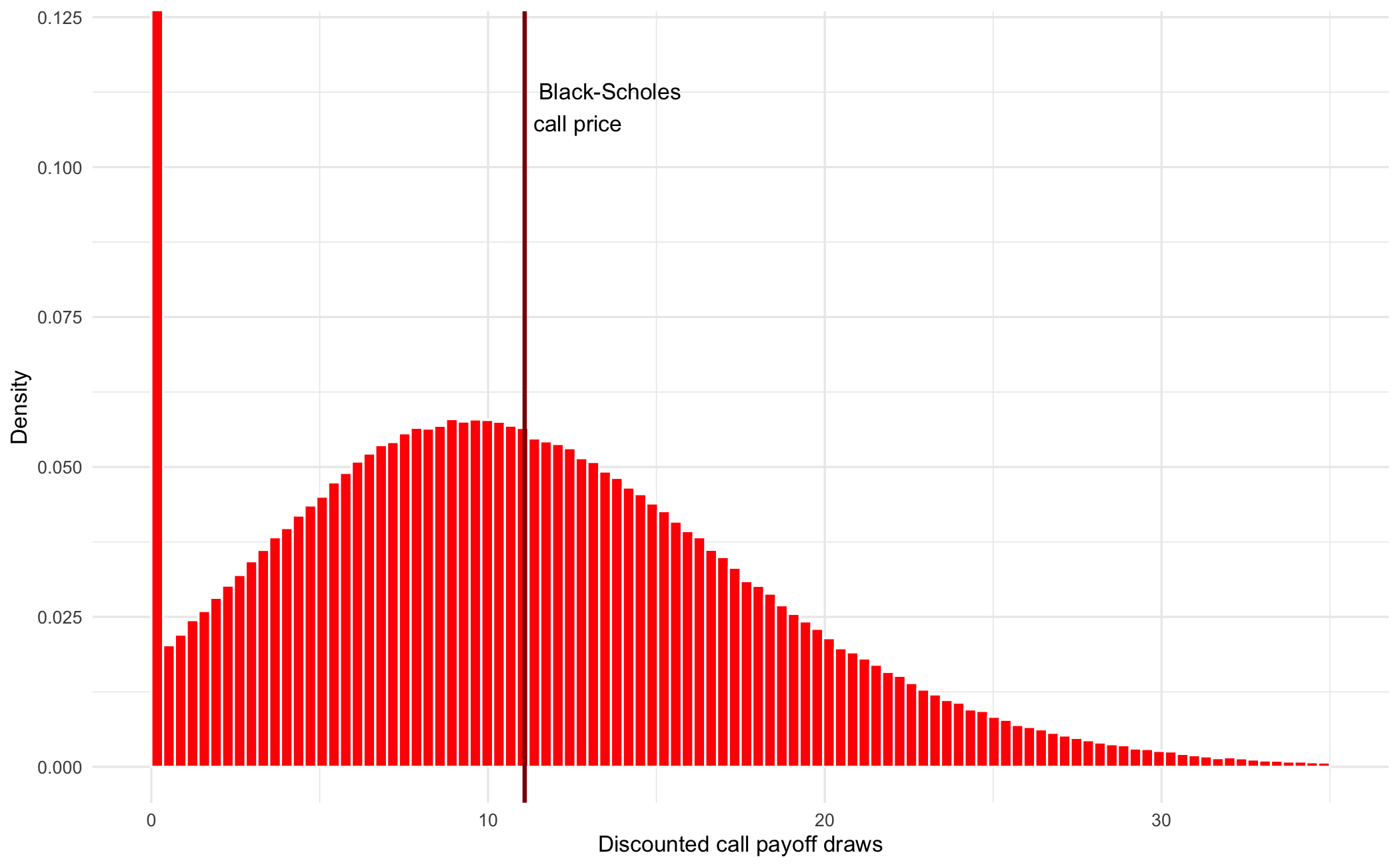
from plotnine import after_stat

fsim = sim()
df_hist = pd.DataFrame({'price': fsim})
breaks = np.linspace(0, 35, 101)

p = (ggplot(df_hist, aes(x='price'))
 + geom_histogram(aes(y=after_stat("density")), breaks=breaks, fill="red", colour="white")
 + geom_vline(xintercept=bsprice['Call'], colour="darkred", size=1)
 + annotate("text", x=bsprice['Call'], y=0.11, label="Black-Scholes\ncall price", ha="left")
 + coord_cartesian(ylim=(0, 0.12))
 + labs(x="Discounted call payoff draws", y="Density")
 + theme_minimal())
p.save("_figs/sim_hist_py.png", width=6, height=4, dpi=100, verbose=False)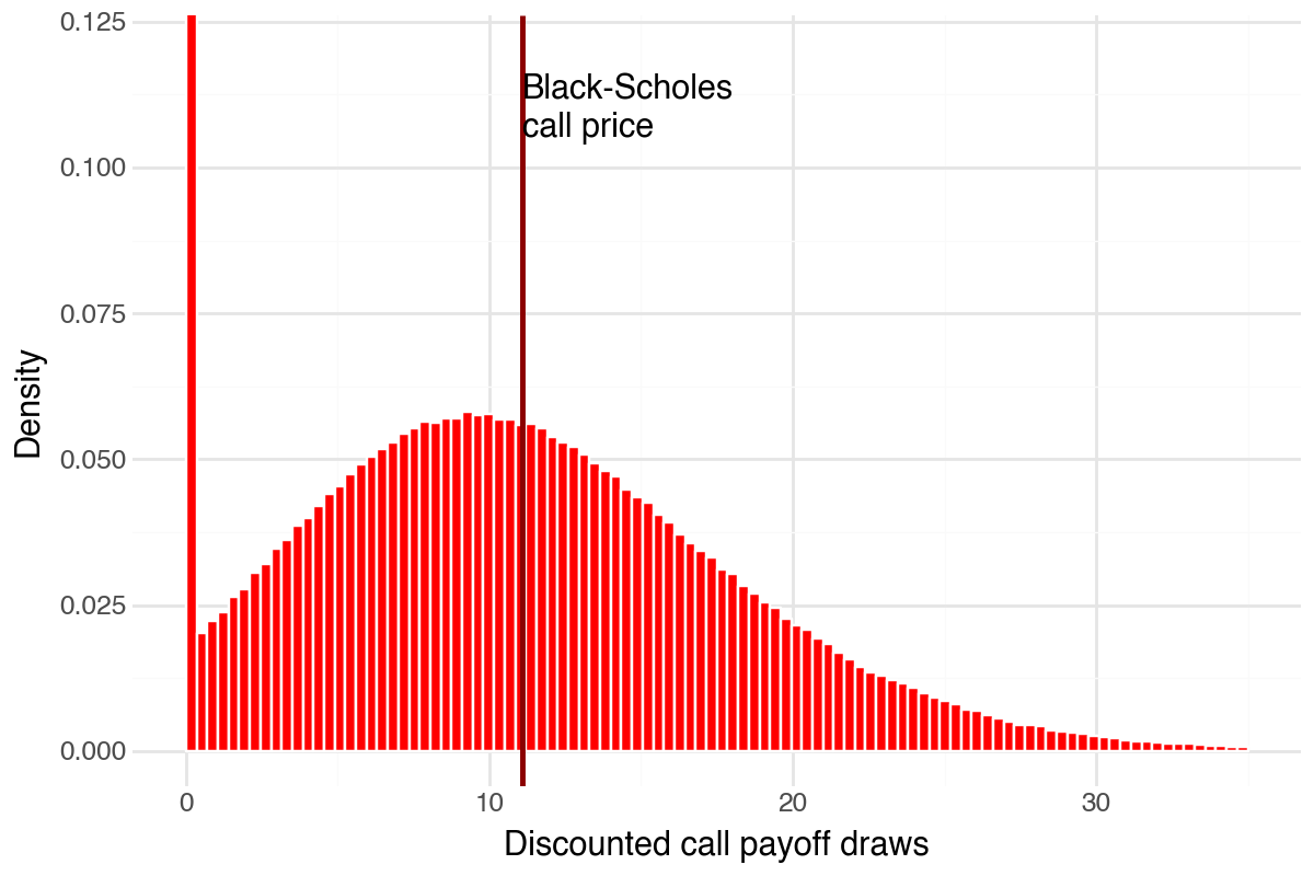
using Random, Distributions, DataFrames, TidierPlots
P0 = 50; sigma = 0.2; r = 0.05; T = 0.5; X = 40;

function sim(S=1000000; P0=50, sigma=0.2, r=0.05, T=0.5, X=40, seed=666)
    Random.seed!(seed);
    F = P0 * exp(r * T);
    ysim = rand(Normal(-0.5 * sigma^2 * T, sigma * sqrt(T)), S);
    F = F .* exp.(ysim);
    SP = max.(F .- X, 0);
    fsim = SP .* exp(-r * T);
    return fsim
end

fsim = sim();
df_hist = DataFrame(price = fsim);

bscall = bsprice.Call;
edges = range(0, 35, length=101);
counts = [count(x -> edges[i] <= x < edges[i+1], fsim) for i in 1:100];
binwidth = edges[2] - edges[1];
density_vals = counts ./ (length(fsim) * binwidth);
mids = [(edges[i] + edges[i+1]) / 2 for i in 1:100];

df_hist_bars = DataFrame(mid = mids, density = density_vals);
df_line = DataFrame(x = [bscall, bscall], y = [0.0, maximum(density_vals)]);
df_label = DataFrame(x = [bscall], y = [maximum(density_vals)], label = ["Black-Scholes\ncall price"]);

p = ggplot(df_hist_bars, @aes(x = mid, y = density)) +
    geom_col(color = "red", width = binwidth) +
    geom_line(@aes(x = x, y = y), data = df_line, color = "darkred", linewidth = 1) +
    geom_text(@aes(x = x, y = y, label = label), data = df_label) +
    labs(x = "Discounted call payoff draws", y = "Density") +
    theme_minimal();
ggsave("_figs/sim_hist_jl.png", p);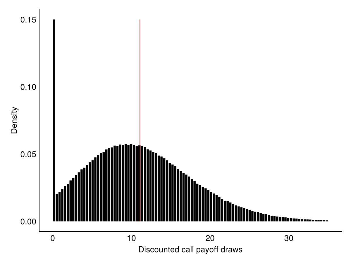
The mean of the discounted payoff draws is the Monte Carlo estimate of the call price. Confidence bounds for that estimate come from the standard error of the mean across draws, not from the spread of the draws themselves. We leave the calculation as an exercise.
Chapter 25 covers further applications of simulation in risk management, including portfolio Value-at-Risk calculations.
15.7 Multivariate simulation
Everything so far has simulated one risk factor. The second application of the same machinery is several at once, where what has to be simulated is not just each series but how they move together.
In a crisis, assets that looked diversified start falling together, and the dependence is stronger on the downside than on the upside. Copulas address this by separating the dependence structure from the marginal distributions, allowing each to be modelled independently. Whether a copula captures joint crashes depends on which one is chosen. The Gaussian copula below has no asymptotic tail dependence, while the Clayton copula produces the lower-tail clustering visible in its scatter plot. We return to multivariate simulation in Chapter 25.
The word asymptotic is doing real work there. Tail dependence is a limit — the probability that one asset breaches its \(\probability\)-quantile given that the other has, as \(\probability \to 0\). For the Gaussian copula with any correlation below one, that limit is zero.
It does not follow that joint losses are rare at the thresholds we actually use. A Gaussian copula with \(\correlation = 0.7\) still puts far more probability on both assets breaching their 1% quantiles together than independence would, and 1% is not the limit. What the zero limit says is that the clustering thins out as we go further into the tail, and eventually behaves as if the assets were independent. The practical question is whether it thins out before or after the loss level we care about.
We start with the multivariate normal. To simulate correlated values:
The library MASS allows us to simulate multivariate normals with mvrnorm.
mu = c(0, 0)
Sigma = matrix(c(1, 0.8, 0.8, 1), ncol = 2)
mv_data = mvrnorm(n = 1000, mu = mu, Sigma = Sigma)
df_mv = data.frame(x = mv_data[, 1], y = mv_data[, 2])

ggplot(df_mv, aes(x = x, y = y)) +
  geom_point(colour = "blue", alpha = 0.5) +
  labs(title = "Multivariate Normal Simulation", x = "", y = "") +
  theme_minimal()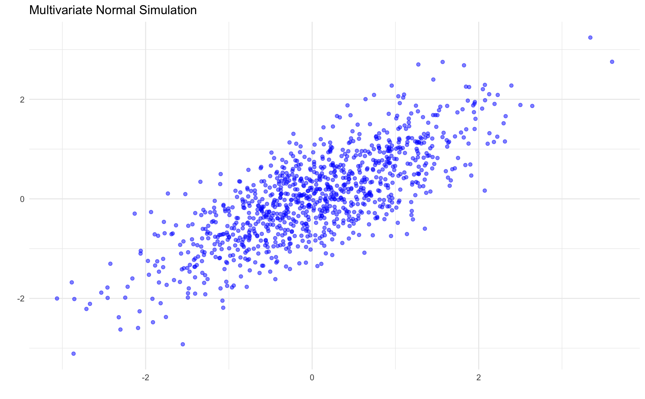
NumPy provides multivariate_normal for correlated simulations.
mu = [0, 0]
cov_matrix = [[1, 0.8], [0.8, 1]]
mv_data = np.random.multivariate_normal(mu, cov_matrix, 1000)
df_mv = pd.DataFrame({'x': mv_data[:, 0], 'y': mv_data[:, 1]})

p = (ggplot(df_mv, aes(x='x', y='y'))
 + geom_point(colour="blue", alpha=0.5)
 + labs(title="Multivariate Normal Simulation", x="", y="")
 + theme_minimal())
p.save("_figs/sim_mv_py.png", width=6, height=4, dpi=100, verbose=False)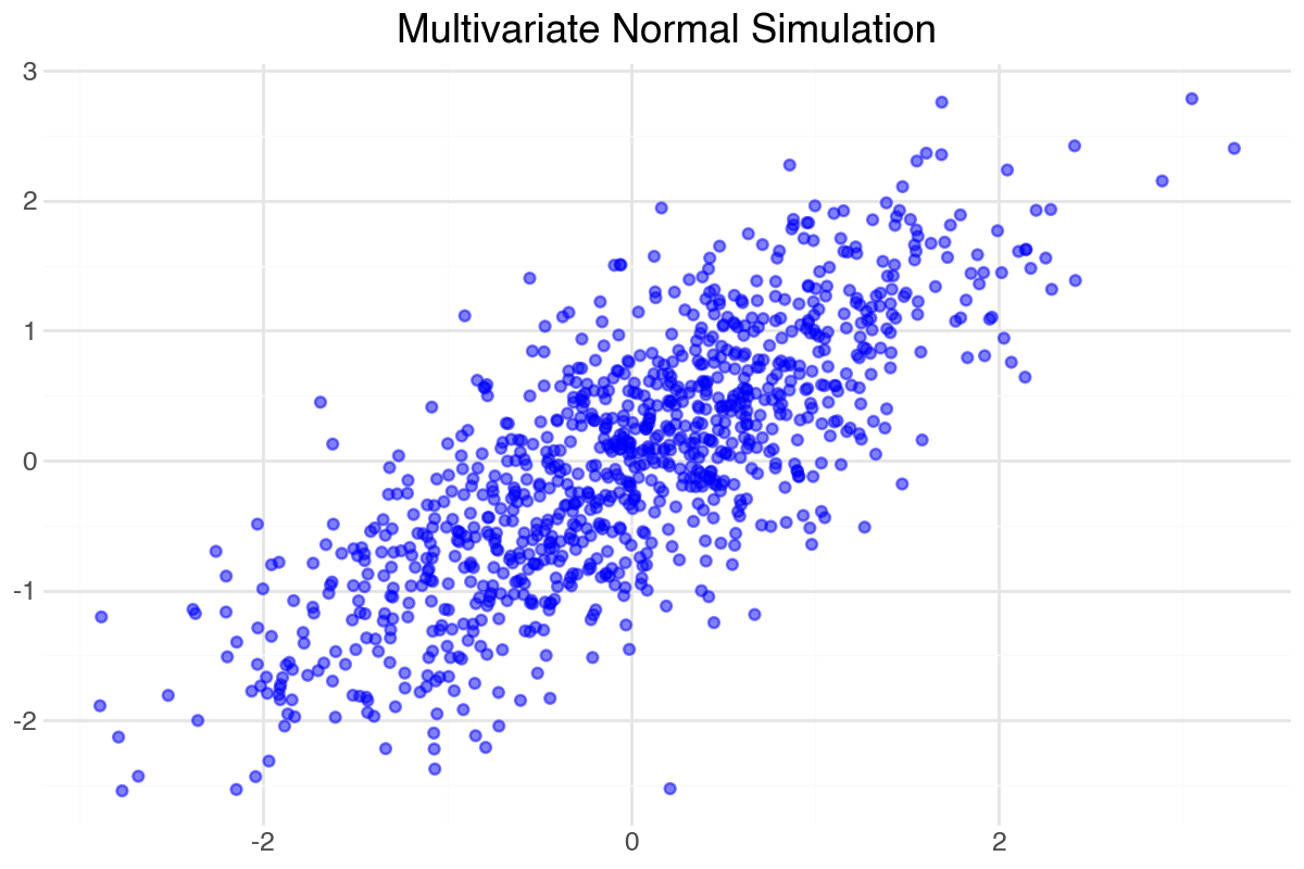
Julia uses MvNormal from Distributions.
mu = [0.0, 0.0];
Sigma = [1.0 0.8; 0.8 1.0];
mv_data = rand(MvNormal(mu, Sigma), 1000)';
df_mv = DataFrame(x = mv_data[:, 1], y = mv_data[:, 2]);

p = ggplot(df_mv, @aes(x = x, y = y)) +
    geom_point(color = "blue", alpha = 0.5) +
    labs(title = "Multivariate Normal Simulation", x = "", y = "") +
    theme_minimal();
ggsave("_figs/sim_mv_jl.png", p);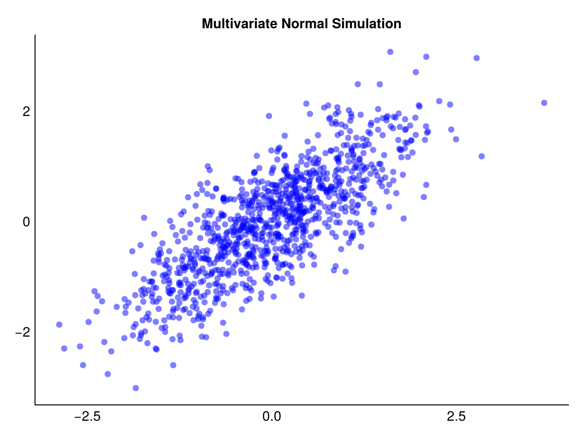
15.7.1 Copulas
A copula lets us model two things separately — how each variable behaves on its own and how the variables move together.
Library copula provides various copula types.
normal_cop = normalCopula(param = 0.7, dim = 2)
cop_sample = rCopula(1000, normal_cop)
df_cop_unif = data.frame(x = cop_sample[, 1], y = cop_sample[, 2])

ggplot(df_cop_unif, aes(x = x, y = y)) +
  geom_point(colour = "purple", alpha = 0.5) +
  labs(title = "Gaussian Copula (uniform margins)", x = "", y = "") +
  theme_minimal()

clayton_cop = claytonCopula(param = 2, dim = 2)
u = rCopula(1000, clayton_cop)
df_clayton = data.frame(U1 = u[, 1], U2 = u[, 2])

ggplot(df_clayton, aes(x = U1, y = U2)) +
  geom_point(colour = "blue", alpha = 0.5) +
  labs(title = "Clayton Copula") +
  theme_minimal()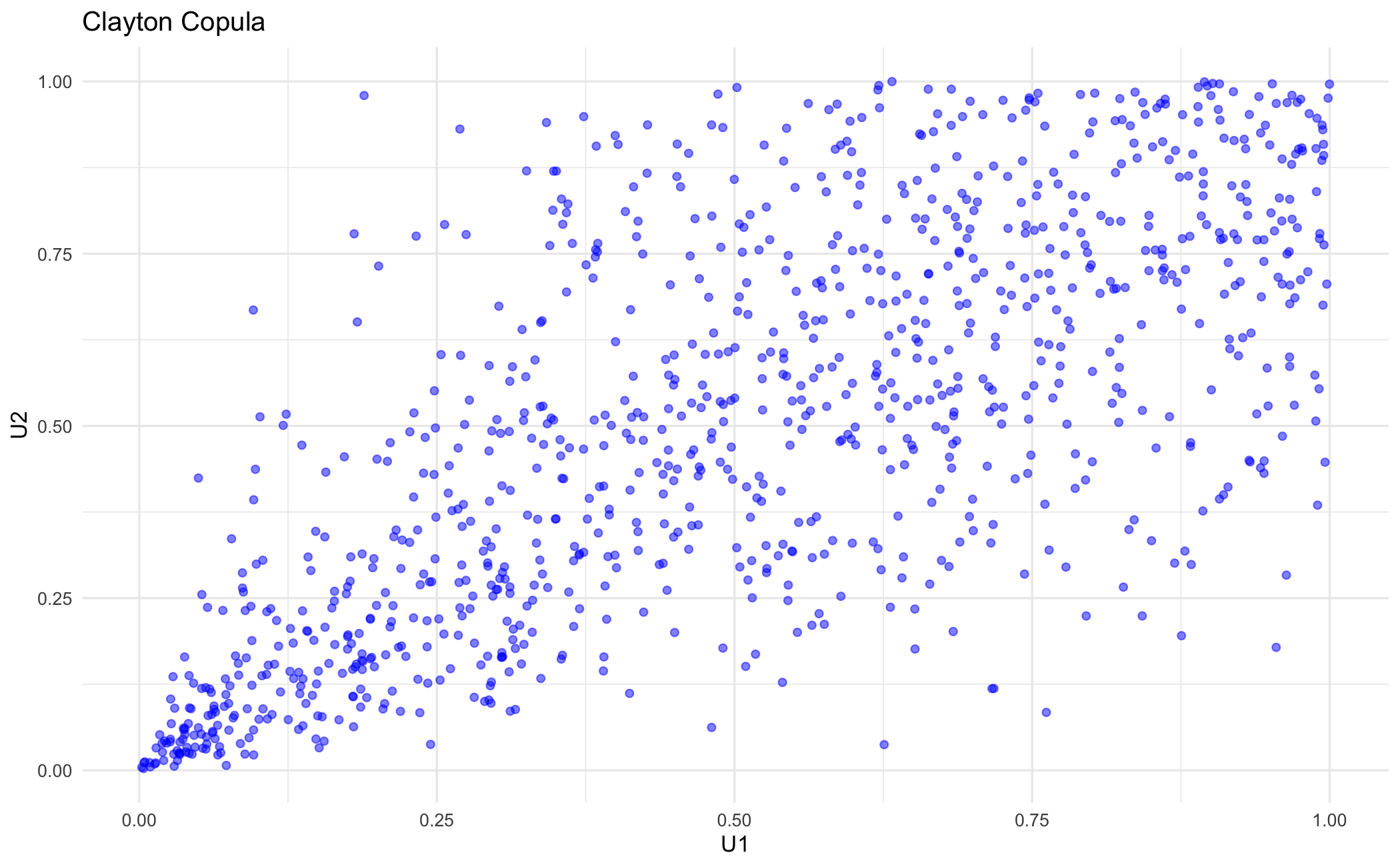
We can construct a Gaussian copula manually using the correlation structure.
# Gaussian copula via correlation
rho = 0.7
z = np.random.multivariate_normal([0, 0], [[1, rho], [rho, 1]], 1000)
u = norm.cdf(z)  # Transform to uniform margins
df_cop = pd.DataFrame({'x': u[:, 0], 'y': u[:, 1]})

p = (ggplot(df_cop, aes(x='x', y='y'))
 + geom_point(colour="purple", alpha=0.5)
 + labs(title="Gaussian Copula (uniform margins)", x="", y="")
 + theme_minimal())
p.save("_figs/sim_cop_py.png", width=6, height=4, dpi=100, verbose=False)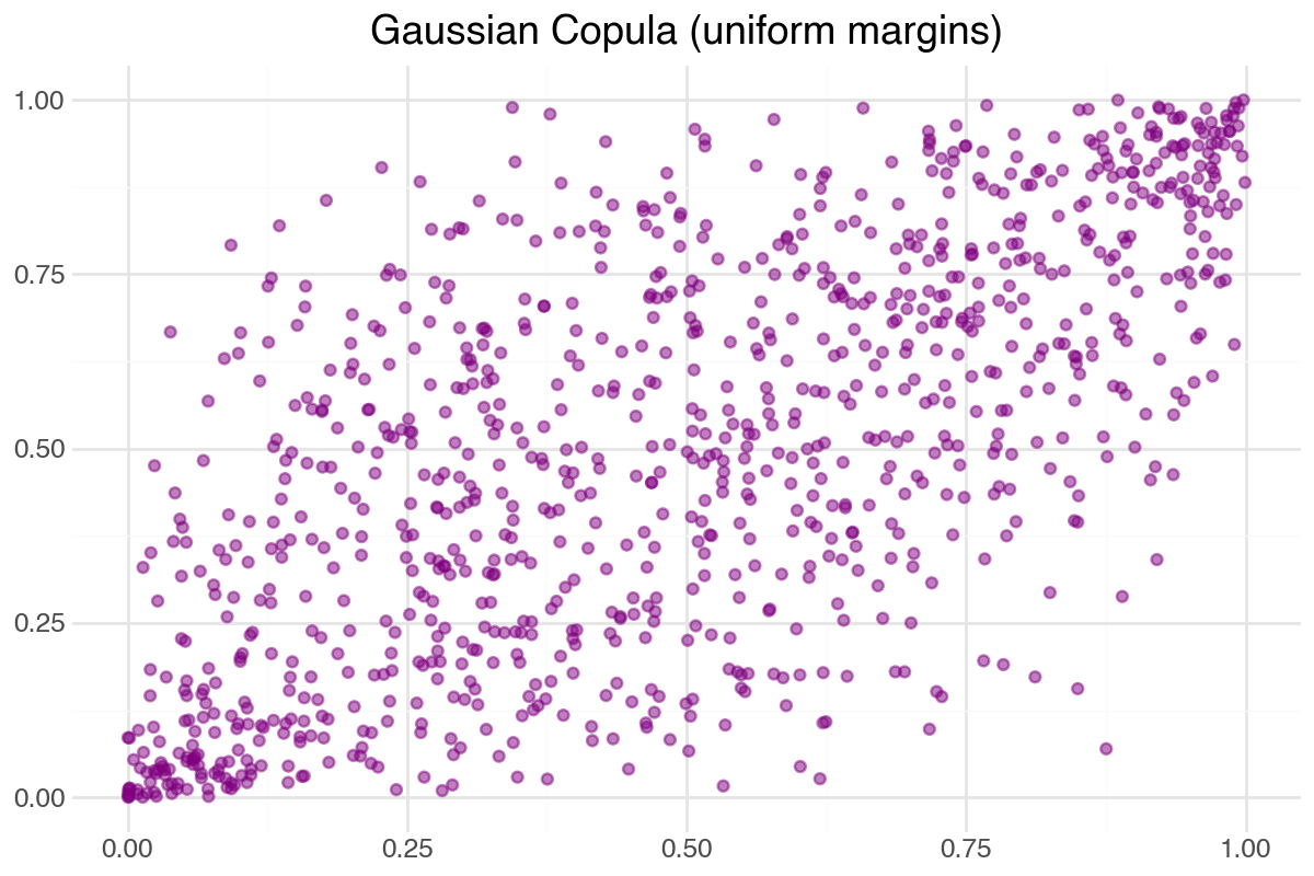
Clayton copula using the conditional distribution method:
# Clayton copula via conditional inverse
theta = 2.0
n = 1000
u1 = np.random.uniform(size=n)
v = np.random.uniform(size=n)
u2 = (u1**(-theta) * (v**(-theta/(theta+1)) - 1) + 1)**(-1/theta)
df_clayton = pd.DataFrame({'U1': u1, 'U2': u2})

p = (ggplot(df_clayton, aes(x='U1', y='U2'))
 + geom_point(colour="blue", alpha=0.5)
 + labs(title="Clayton Copula")
 + theme_minimal())
p.save("_figs/sim_clayton_py.png", width=6, height=4, dpi=100, verbose=False)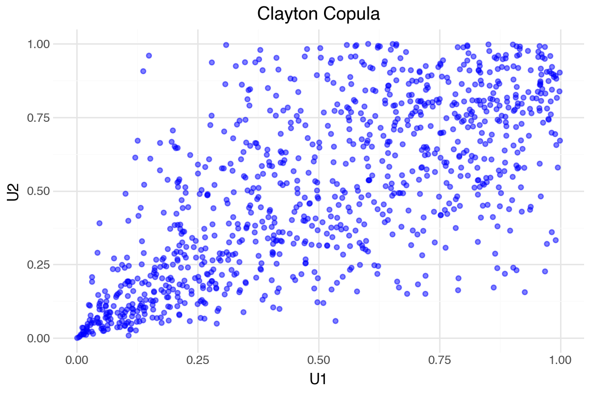
# Gaussian copula via correlation
rho = 0.7;
Sigma = [1.0 rho; rho 1.0];
z = rand(MvNormal([0.0, 0.0], Sigma), 1000)';
u = cdf.(Normal(), z);
df_cop = DataFrame(x = u[:, 1], y = u[:, 2]);

p = ggplot(df_cop, @aes(x = x, y = y)) +
    geom_point(color = "purple", alpha = 0.5) +
    labs(title = "Gaussian Copula (uniform margins)", x = "", y = "") +
    theme_minimal();
ggsave("_figs/sim_cop_jl.png", p);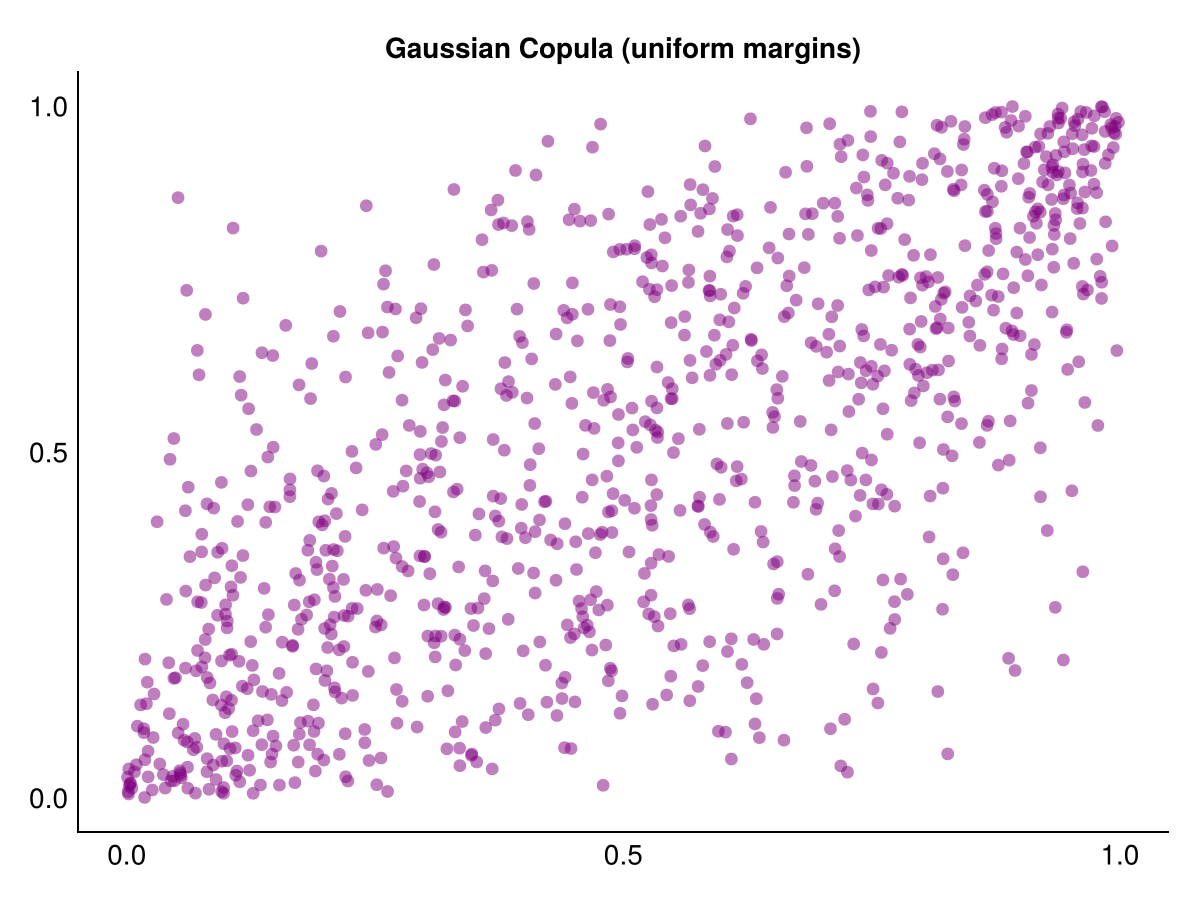
Clayton copula using Copulas.jl:
clayton = ClaytonCopula(2, 2.0);
u = rand(clayton, 1000)';
df_clayton = DataFrame(U1 = u[:, 1], U2 = u[:, 2]);

p = ggplot(df_clayton, @aes(x = U1, y = U2)) +
    geom_point(color = "blue", alpha = 0.5) +
    labs(title = "Clayton Copula") +
    theme_minimal();
ggsave("_figs/sim_clayton_jl.png", p);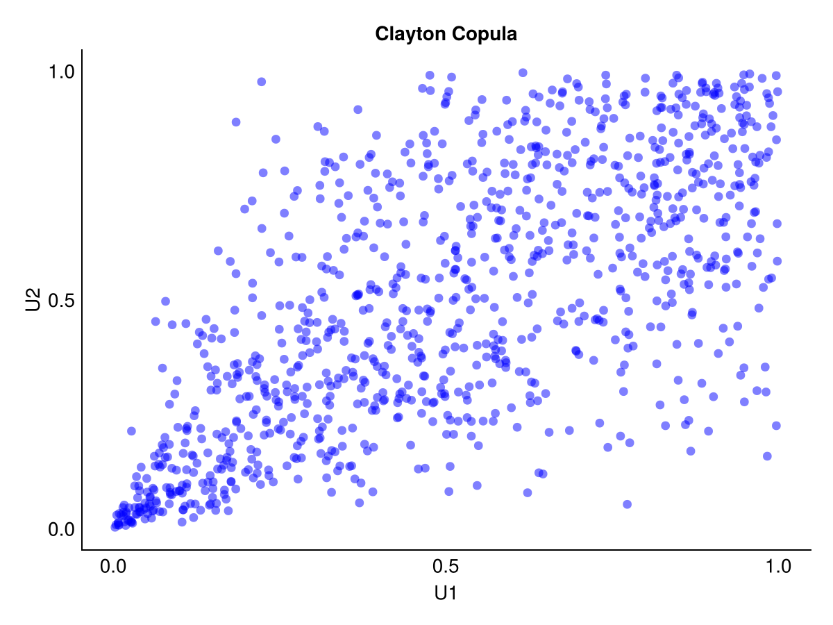
15.8 Exercise
- Use simulations to get the confidence bounds for the simulation estimates.
- Draw from the Clayton copula at a range of dependence parameters and count how often both series breach their 1% quantile on the same draw. Compare with the Gaussian copula at the correlation that produces the same overall dependence.