library(lubridate)
library(zoo)
library(reshape2)
library(car)
library(tseries)
source("common/functions.r", chdir = TRUE)
library(tsgarch)
library(xts)
library(ggplot2)19 Evaluating volatility models
Chapter 18 fitted four specifications and read their diagnostics. Neither exercise settles which model to run. A model can pass its residual tests and still generate paths that look nothing like the data, and it can sit closely on the estimation sample and forecast badly outside it.
This chapter asks both questions. Simulation shows what a fitted model implies, by drawing paths from it and setting them beside the returns it was fitted to. Out-of-sample evaluation scores its forecasts on days the estimation never touched. A specification can pass one and fail the other.
19.1 Data and libraries
The same libraries as the previous chapter, and the same S&P 500 returns.
import numpy as np
import pandas as pd
import sys
sys.path.insert(0, 'common')
from functions import ProcessRawData
from arch import arch_model
from plotnine import ggplot, aes, geom_line, labs, theme_minimal
using CSV, DataFrames, Dates, Statistics
using ARCHModels
using TidierPlots, CairoMakie
using Distributions
using StatsBase
using HypothesisTests
using Random
using Printf
include("common/functions.jl");data = ProcessRawData()
dates = as.Date(as.character(data$sp500$date), format="%Y%m%d")
y = xts(data$sp500$y, order.by = dates)
y = na.omit(y)
y = y - mean(y)
y = y * 100data = ProcessRawData()
y = data['sp500']['y'].values
y = y[~np.isnan(y)]
y = y - np.mean(y)
y = y * 100data = ProcessRawData();
y = collect(skipmissing(data["sp500"].y));
y = y .- mean(y);
y = y .* 100;19.2 Monte Carlo analysis of GARCH models
A fitted GARCH is a recipe for generating returns. Running that recipe forward and looking at what comes out is the most direct check there is on whether the model describes the data, and it catches things the residual tests do not.
19.2.1 Using simulate()
The code in this section and the next is shown but not run, so no output or figures appear below it. Each tab draws a 5,000 observation path from the fitted GARCH-t and plots it beside the S&P 500 returns, which makes it easy to see how much of the appearance of the data the model reproduces.
spec_sim = garch_modelspec(y = y, model = "garch", order = c(1, 1), distribution = "std")
spec_sim$parmatrix$value[match(Results$tGARCH11$parmatrix$parameter, spec_sim$parmatrix$parameter)] = Results$tGARCH11$parmatrix$value
s = simulate(spec_sim, nsim = 1, h = 5000)
sim_series = as.numeric(s$series[1, ])
sim_xts = xts(sim_series, order.by = seq(as.Date("2000-01-01"), by = "day", length.out = length(sim_series)))

par(mar = c(2, 3, 2, 0))
plot(y, type = 'l', bty = 'l', las = 1, main = "S&P 500")
plot(sim_xts, type = 'l', bty = 'l', las = 1, main = "Simulated GARCH-t S&P 500")
sim = Results['tGARCH11'].model.simulate(Results['tGARCH11'].params, nobs=5000)
df_obs = pd.DataFrame({'t': range(len(y)), 'y': y})
p = (ggplot(df_obs, aes(x='t', y='y'))
+ geom_line(size=0.5)
+ labs(title='S&P 500', x='', y='')
+ theme_minimal())
p.save("_figs/sim_obs_py.png", width=10, height=4, dpi=100)
df_sim = pd.DataFrame({'t': range(len(sim['data'])), 'y': sim['data']})
p = (ggplot(df_sim, aes(x='t', y='y'))
+ geom_line(size=0.5)
+ labs(title='Simulated GARCH-t S&P 500', x='', y='')
+ theme_minimal())
p.save("_figs/sim_tgarch_py.png", width=10, height=4, dpi=100)using ARCHModels, DataFrames, TidierPlots
df_obs = DataFrame(t = 1:length(y), y = y)
p = ggplot(df_obs, @aes(x = t, y = y)) +
geom_line() +
labs(title = "S&P 500", x = "", y = "Returns")
ggsave("_figs/sim_obs_jl.png", p)
sim = simulate(Results_jl["tGARCH11"], 5000)
df_sim = DataFrame(t = 1:length(sim.data), y = sim.data)
p = ggplot(df_sim, @aes(x = t, y = y)) +
geom_line() +
labs(title = "Simulated GARCH-t S&P 500", x = "", y = "Returns")
ggsave("_figs/sim_tgarch_jl.png", p)19.2.1.1 Simulation and estimation
Simulating from a fitted model and re-estimating on the simulated data is a check on the estimator. If the code is right, the coefficients recovered from each simulated path should scatter around the parameters that generated it. Watch how much they move from one path to the next, because that spread is the sampling uncertainty in the original estimates.
N = 5
for (n in 1:N) {
  spec_sim = garch_modelspec(y = y, model = "garch", order = c(1, 1), distribution = "norm")
  spec_sim$parmatrix$value[match(Results$GARCH11$parmatrix$parameter, spec_sim$parmatrix$parameter)] = Results$GARCH11$parmatrix$value
  s = simulate(spec_sim, nsim = 1, h = 5000)
  sim_series = as.numeric(s$series[1, ])
  sim_xts = xts(sim_series, order.by = seq(as.Date("2000-01-01"), by = "day", length.out = length(sim_series)))
  spec_re = garch_modelspec(y = sim_xts, model = "garch", order = c(1, 1), distribution = "norm")
  fit_sim = estimate(spec_re)
  print(coef(fit_sim))
}
N = 5
for n in range(N):
sim = Results['GARCH11'].model.simulate(Results['GARCH11'].params, nobs=5000)
model = arch_model(sim['data'], vol='GARCH', p=1, q=1, dist='normal', mean='Zero')
fit = model.fit(disp='off')
print(fit.params.values)using ARCHModels
N = 5
for n in 1:N
sim = simulate(Results_jl["GARCH11"], 5000)
fit_sim = fit(GARCH{1,1}, sim.data; meanspec=NoIntercept)
println(coef(fit_sim))
end19.2.2 Manual simulation
Package functions are convenient, but writing the recursion out by hand matters. It shows exactly how the process works.
19.2.2.1 GARCH(1,1)
R, Python and Julia use different random number generators, so the simulated paths differ even with the same seed. All three implementations are correct. They simply draw different samples from the same GARCH process.
S = 1e3
omega = 0.02
alpha = 0.15
beta = 0.8

set.seed(42)
eps = rnorm(S)
y_sim = rep(NA, S)
sigma2 = omega / (1 - alpha - beta)

y_sim[1] = eps[1] * sqrt(sigma2)
for (i in 2:S) {
  sigma2 = omega + alpha * y_sim[i-1]^2 + beta * sigma2
  y_sim[i] = eps[i] * sqrt(sigma2)
}

df_sim = data.frame(t = 1:length(y_sim), y = y_sim)
ggplot(df_sim, aes(x = t, y = y)) +
  geom_line() +
  theme_minimal()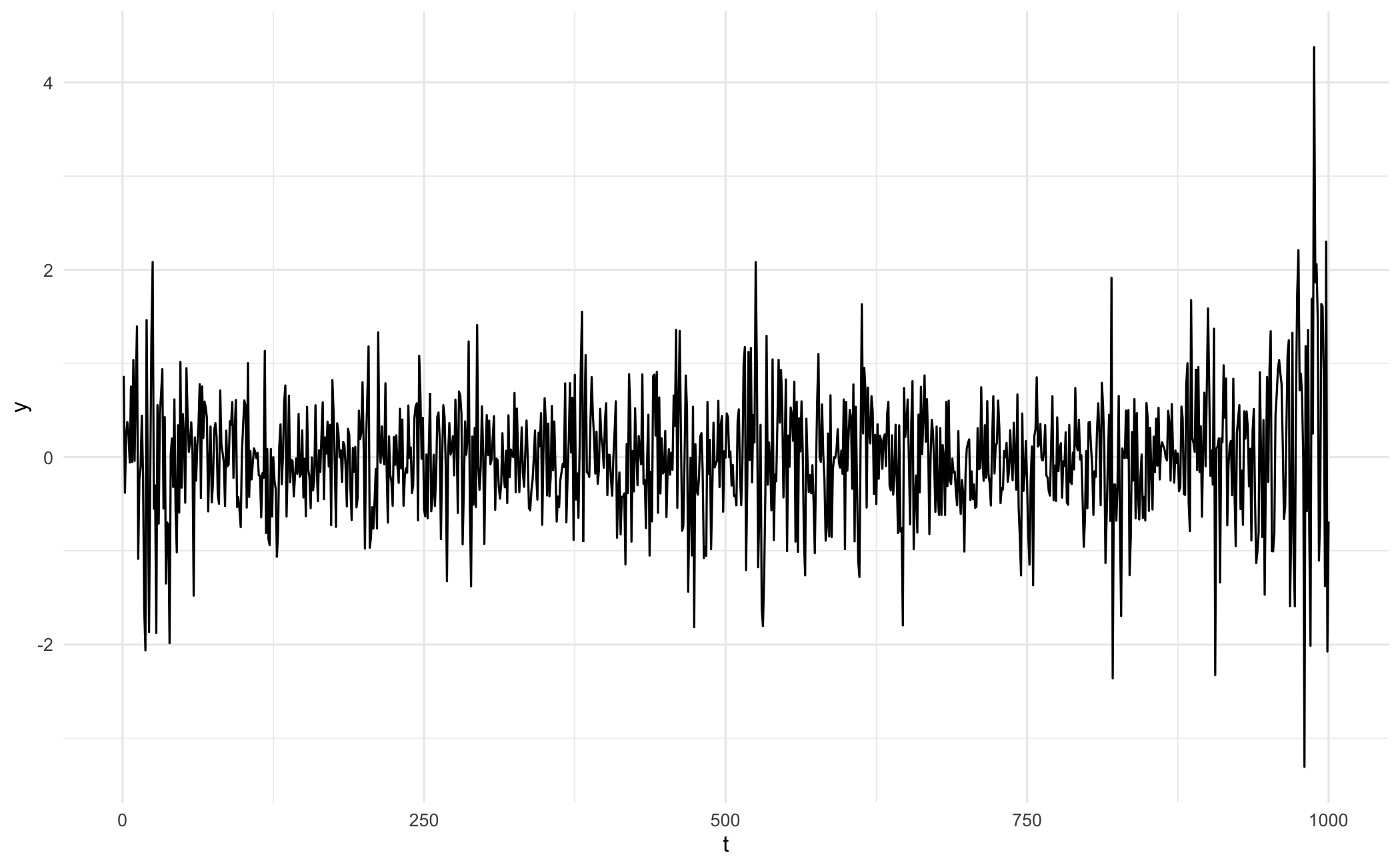
S = 1000
omega = 0.02
alpha = 0.15
beta = 0.8

np.random.seed(42)
eps = np.random.normal(size=S)
y_sim = np.zeros(S)
sigma2 = omega / (1 - alpha - beta)

y_sim[0] = eps[0] * np.sqrt(sigma2)
for i in range(1, S):
    sigma2 = omega + alpha * y_sim[i-1]**2 + beta * sigma2
    y_sim[i] = eps[i] * np.sqrt(sigma2)

df_sim = pd.DataFrame({'t': range(len(y_sim)), 'y': y_sim})
p = (ggplot(df_sim, aes(x='t', y='y'))
 + geom_line(size=0.5)
 + theme_minimal())
p.save("_figs/vol_sim_garch_py.png", width=10, height=3, dpi=100)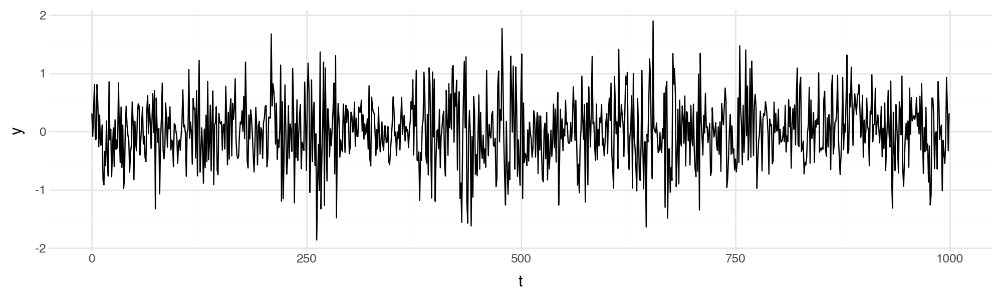
function simulate_garch(S, omega, alpha, beta, seed)
    Random.seed!(seed)
    eps = randn(S)
    y = zeros(S)
    sigma2 = omega / (1 - alpha - beta)

    y[1] = eps[1] * sqrt(sigma2)
    for i in 2:S
        sigma2 = omega + alpha * y[i-1]^2 + beta * sigma2
        y[i] = eps[i] * sqrt(sigma2)
    end
    return y
end

y_sim = simulate_garch(1000, 0.02, 0.15, 0.8, 42);
df_sim = DataFrame(t = 1:length(y_sim), y = y_sim);
p = ggplot(df_sim, @aes(x = t, y = y)) +
    geom_line(linewidth = 0.3) +
    labs(x = "", y = "") +
    theme_minimal();
ggsave("_figs/vol_sim_garch_jl.png", p);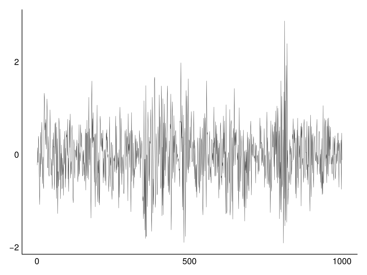
19.2.2.2 GARCH-t
The same recursion with Student-t innovations. Only the draw changes — the variance equation is identical — and the standardisation by \(\sqrt{\DOF/(\DOF-2)}\) keeps the innovations at unit variance so \(\GARCHconst\), \(\ARCHcoeff\) and \(\GARCHcoeff\) mean what they meant before.
df = 6
omega = 0.02
alpha = 0.15
beta = 0.75
S = 1e4

set.seed(42)
eps = rt(S, df = df) / sqrt(df / (df - 2))
y_sim = rep(NA, S)
sigma2 = omega / (1 - alpha - beta)

y_sim[1] = eps[1] * sqrt(sigma2)
for (i in 2:S) {
  sigma2 = omega + alpha * y_sim[i-1]^2 + beta * sigma2
  y_sim[i] = eps[i] * sqrt(sigma2)
}

df_sim = data.frame(t = 1:length(y_sim), y = y_sim)
ggplot(df_sim, aes(x = t, y = y)) +
  geom_line() +
  theme_minimal()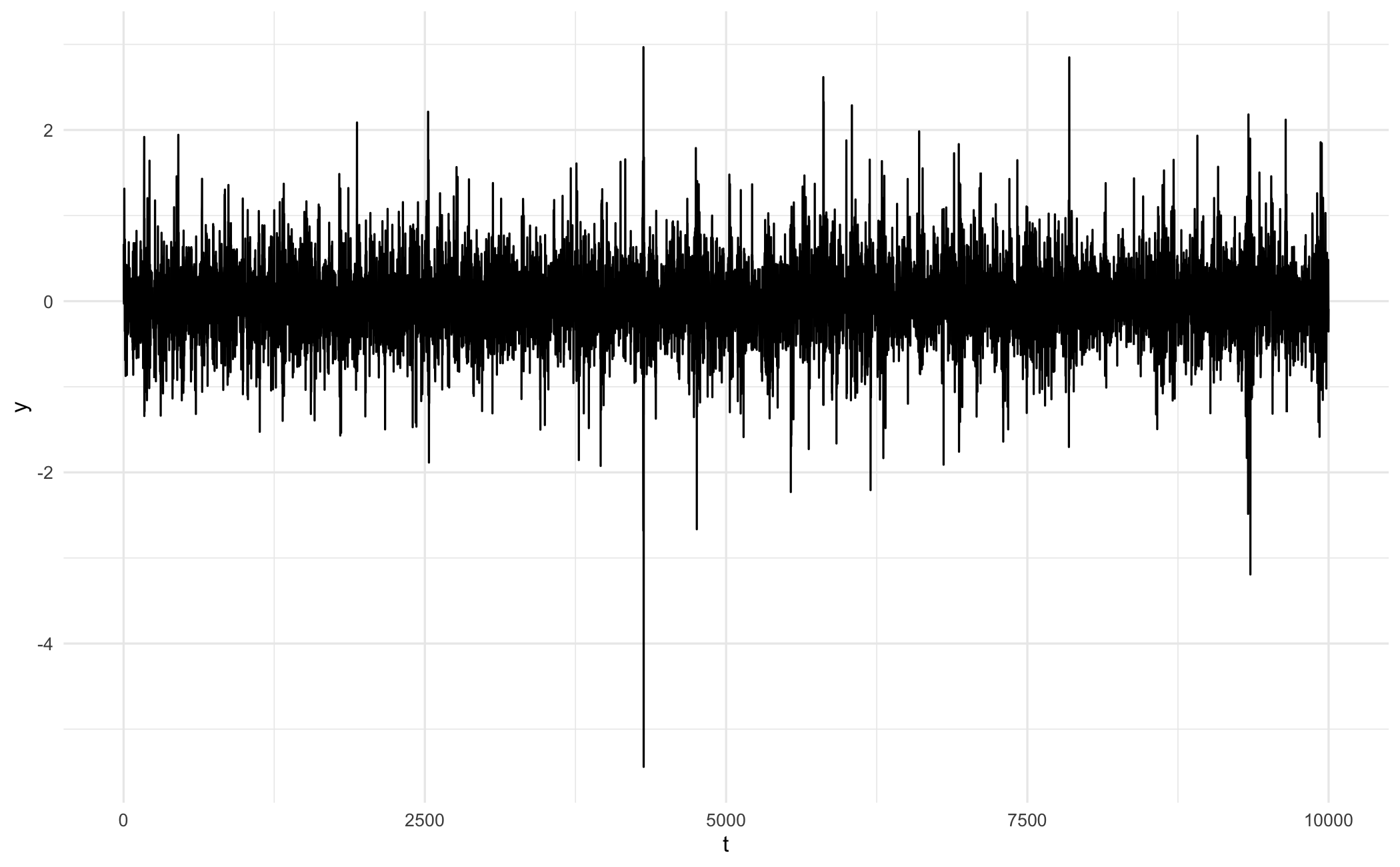
df = 6
omega = 0.02
alpha = 0.15
beta = 0.75
S = 10000

np.random.seed(42)
eps = np.random.standard_t(df, size=S) / np.sqrt(df / (df - 2))
y_sim = np.zeros(S)
sigma2 = omega / (1 - alpha - beta)

y_sim[0] = eps[0] * np.sqrt(sigma2)
for i in range(1, S):
    sigma2 = omega + alpha * y_sim[i-1]**2 + beta * sigma2
    y_sim[i] = eps[i] * np.sqrt(sigma2)

df_sim = pd.DataFrame({'t': range(len(y_sim)), 'y': y_sim})
p = (ggplot(df_sim, aes(x='t', y='y'))
 + geom_line(size=0.5)
 + theme_minimal())
p.save("_figs/vol_sim_tgarch_py.png", width=10, height=3, dpi=100)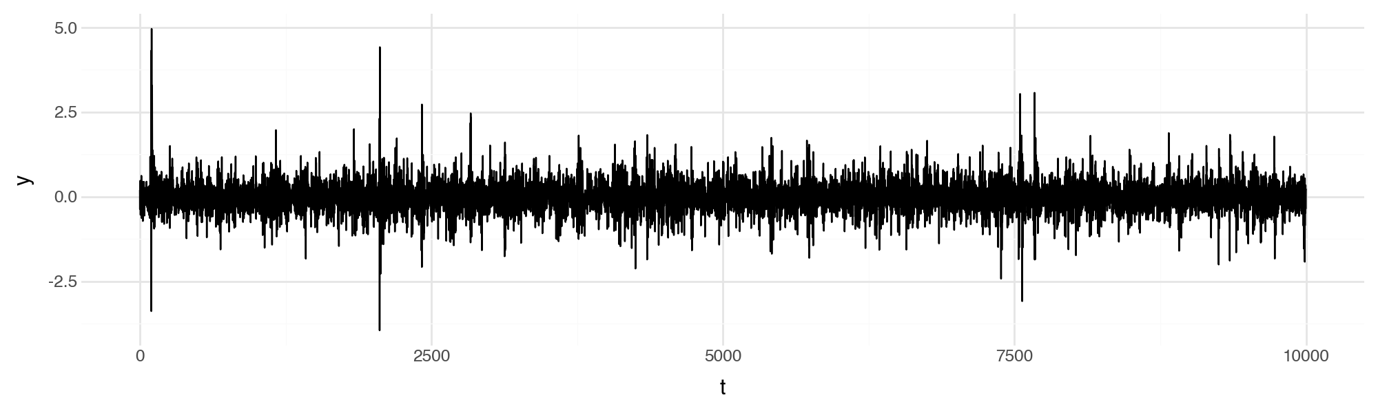
function simulate_tgarch(S, omega, alpha, beta, df, seed)
    Random.seed!(seed)
    eps = rand(TDist(df), S) ./ sqrt(df / (df - 2))
    y = zeros(S)
    sigma2 = omega / (1 - alpha - beta)

    y[1] = eps[1] * sqrt(sigma2)
    for i in 2:S
        sigma2 = omega + alpha * y[i-1]^2 + beta * sigma2
        y[i] = eps[i] * sqrt(sigma2)
    end
    return y
end

y_sim = simulate_tgarch(10000, 0.02, 0.15, 0.75, 6, 42);
df_sim = DataFrame(t = 1:length(y_sim), y = y_sim);
p = ggplot(df_sim, @aes(x = t, y = y)) +
    geom_line(linewidth = 0.3) +
    labs(x = "", y = "") +
    theme_minimal();
ggsave("_figs/vol_sim_tgarch_jl.png", p);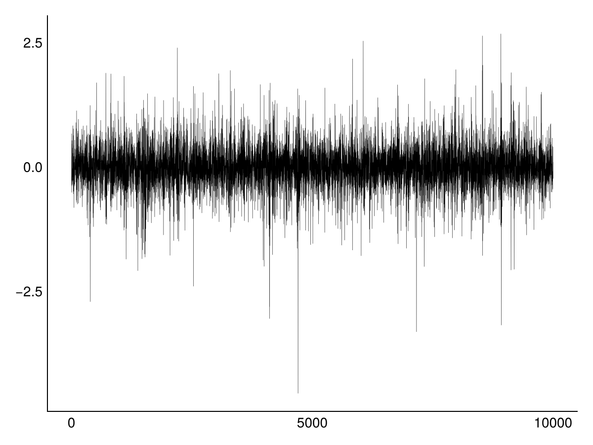
19.3 Out-of-sample forecast evaluation
Everything so far judges a model by how snugly it sits on the sample used to estimate it. Likelihood, AIC and BIC all work that way. But fitting the past closely and predicting the future well are different skills, and it is the second one we are buying. So the comparison that settles which specification to run should be made on days the estimation never touched.
The scheme is the one the backtesting chapter uses — estimate on a rolling window, record the one-step-ahead variance forecast, roll forward, repeat. What is different here is the scoring, and it runs into an immediate problem — volatility is not observed, so there is nothing to compare the forecast against.
Something observable has to stand in for it. The squared return is the natural candidate, and it is unbiased, but the substitution is a poor one day by day. Write \(\CompoundReturns_t^2 = \Vol_t^2 \StdNormal_t^2\). The thing we want is multiplied by a random factor whose mean is one and whose variance, under normality, is two. One day’s squared return is therefore a wildly dispersed reading of that day’s variance.
Intraday data supports a much sharper proxy, since summing squared five-minute returns averages the noise away, and that is the route to take when such data is to hand. It is not here, so we use squared returns and rely on the evaluation period being long enough for the dispersion to average out across days. That is enough to rank two models. It would not be enough to say anything about one particular Tuesday.
Two loss functions are standard. Writing \(\hat{\Vol}_t^2\) for the forecast and \(\tilde{\Vol}_t^2\) for the proxy,
\[L^{\mathrm{MSE}}_t = \left(\hat{\Vol}_t^2 - \tilde{\Vol}_t^2\right)^2, \qquad L^{\mathrm{QLIKE}}_t = \log \hat{\Vol}_t^2 + \frac{\tilde{\Vol}_t^2}{\hat{\Vol}_t^2},\]
each averaged over the evaluation period, lower being better. They are not interchangeable. MSE works on the difference of two variances, so it is symmetric and, being squared, is driven by whichever days happen to be largest.
QLIKE is asymmetric, and the reason is exact. Subtract \(\log \tilde{\Vol}_t^2\), which the forecast cannot influence and which therefore changes no ranking. What is left depends on the forecast only through the ratio \(\rho_t = \tilde{\Vol}_t^2 / \hat{\Vol}_t^2\) of actual to forecast:
\[L^{\mathrm{QLIKE}}_t - \log \tilde{\Vol}_t^2 = \rho_t - \log \rho_t .\]
That function bottoms out at \(\rho_t = 1\) and climbs away from it unevenly. Forecasting half the variance that arrives, \(\rho_t = 2\), costs about 0.31. Forecasting twice what arrives, \(\rho_t = 1/2\), costs about 0.19. So the penalty attaches to getting the ratio wrong, in either direction, but it bites harder when the forecast is too low — which is the useful asymmetry for risk work, where the expensive error is being caught short. The penalty does not depend on whether \(\hat{\Vol}_t^2\) is large or small in absolute terms, only on how far the ratio sits from one.
Both losses also have a property that many reasonable-looking alternatives lack. Because the proxy is noisy, a badly chosen loss can end up rewarding models that track the noise instead of the variance, and can rank two models differently from how it would rank them against the true variance. MSE and QLIKE are immune to that. Their expected ranking is the same whether the proxy is noisy or exact (Patton 2011). Scoring on absolute rather than squared errors, or on the volatility scale rather than the variance scale, generally is not.
WE_oos = 1000
n_oos = 250
start_oos = length(y) - n_oos

fc = matrix(NA_real_, nrow = n_oos, ncol = 2,
            dimnames = list(NULL, c("EWMA", "GARCH")))
actual = numeric(n_oos)

for (i in 1:n_oos) {
    win_xts = y[(start_oos + i - WE_oos):(start_oos + i - 1)]  # tsgarch needs xts
    win = as.numeric(win_xts)

    # EWMA: recursion through the window, one-step-ahead forecast
    s2 = var(win)
    for (j in 2:length(win)) s2 = 0.94 * s2 + 0.06 * win[j - 1]^2
    fc[i, "EWMA"] = 0.94 * s2 + 0.06 * win[length(win)]^2

    # GARCH(1,1), refit each step
    spec = garch_modelspec(win_xts, model = "garch", constant = FALSE,
                           order = c(1, 1), distribution = "norm")
    gfit = estimate(spec)
    fc[i, "GARCH"] = as.numeric(predict(gfit, h = 1)$sigma)^2

    actual[i] = as.numeric(y[start_oos + i])^2
}

loss = data.frame(
    Model = colnames(fc),
    MSE   = apply(fc, 2, function(f) mean((f - actual)^2)),
    QLIKE = apply(fc, 2, function(f) mean(log(f) + actual / f))
)
print(loss, row.names = FALSE, digits = 5)
Model MSE QLIKE
EWMA 36.159 1.2870
GARCH 35.822 1.1825WE_oos = 1000
n_oos = 250
start_oos = len(y) - n_oos
fc = {'EWMA': np.empty(n_oos), 'GARCH': np.empty(n_oos)}
actual = np.empty(n_oos)
for i in range(n_oos):
window = y[start_oos + i - WE_oos:start_oos + i]
s2 = np.var(window, ddof=1)
for j in range(1, len(window)):
s2 = 0.94 * s2 + 0.06 * window[j - 1]**2
fc['EWMA'][i] = 0.94 * s2 + 0.06 * window[-1]**2
res = arch_model(window, mean='Zero', vol='GARCH', p=1, q=1, dist='normal').fit(disp='off')
fc['GARCH'][i] = res.forecast(horizon=1, reindex=False).variance.values[-1, 0]
actual[i] = y[start_oos + i]**2
print(f"{'Model':<8} {'MSE':>12} {'QLIKE':>12}")
for m, f in fc.items():
print(f"{m:<8} {np.mean((f - actual)**2):>12.5f} {np.mean(np.log(f) + actual / f):>12.5f}")Model MSE QLIKE
EWMA 36.15949 1.28702
GARCH 35.89600 1.18478WE_oos = 1000
n_oos = 250
start_oos = length(y) - n_oos
fc = Dict("EWMA" => zeros(n_oos), "GARCH" => zeros(n_oos))
actual = zeros(n_oos)
for i in 1:n_oos
window = y[(start_oos + i - WE_oos):(start_oos + i - 1)]
s2 = var(window)
for j in 2:length(window)
s2 = 0.94 * s2 + 0.06 * window[j-1]^2
end
fc["EWMA"][i] = 0.94 * s2 + 0.06 * window[end]^2
gfit = fit(GARCH{1,1}, window; meanspec = NoIntercept)
fc["GARCH"][i] = predict(gfit, :variance)
actual[i] = y[start_oos + i]^2
end
@printf("%-8s %12s %12s\n", "Model", "MSE", "QLIKE")
for m in ["EWMA", "GARCH"]
f = fc[m]
@printf("%-8s %12.5f %12.5f\n", m, mean((f .- actual).^2), mean(log.(f) .+ actual ./ f))
endModel MSE QLIKE
EWMA 36.15949 1.28702
GARCH 35.82430 1.18245One model coming out ahead on average is suggestive, not conclusive. Both were scored on the same days, so the gap between their averages is itself a random quantity, and we should ask whether it is distinguishable from zero. The daily loss differences are not independent — volatility persists, so a stretch of days where one model does better tends to come in a run — which the standard error has to accommodate. That is the Diebold-Mariano test of Section 27.10.4, used here on variance forecasts instead of on VaR.
The exercise has limits. Winning on QLIKE means a model tracked the variance proxy well. It does not mean the model will behave when we start reading quantiles off it. Chapter 26 judges these same forecasts by how often and in what pattern they are breached, which is the question a risk committee and a regulator ask, and the two verdicts can disagree. A specification can score well here and still bunch its violations together.
This also gives a principled way to choose the EWMA decay factor rather than accepting 0.94 by convention. Run the same loop over a grid of \(\EWMAdecay\) and take the value that minimises out-of-sample QLIKE.
19.4 Exercises
- Forecasting evaluation: Generate one-step-ahead volatility forecasts for the last 100 observations and compare forecast accuracy across different model specifications.
Patton, Andrew J. 2011. “Volatility Forecast Comparison Using Imperfect Volatility Proxies.” Journal of Econometrics 160 (1): 246–56.