library(lubridate)
library(ggplot2)
library(reshape2)27 Testing backtests
Counting violations is not enough. A risk model is only useful if failures arrive at the right rate and in the right pattern.
This chapter applies the tests from Chapter 8 of Financial Risk Forecasting to the backtest generated in Chapter 26.
We implement the Christoffersen (1998) testing framework for VaR validation and a simplified version of the Acerbi and Székely (2019) test for ES.
27.1 Data and libraries
The tests need no special packages. What matters is the saved backtest, loaded below.
import numpy as np
import pandas as pd
import pickle
from scipy import stats
using Statistics, Distributions, DataFrames
using Serialization27.2 Loading backtest data
We load the backtesting results generated in Chapter 26. Each language loads from its native binary format. The saved files include the backtest data, the parameters used and metadata about when and where the backtest was run.
stale_msg = "Risk/backtest.* is stale or missing - re-run the backtest workflow in the Backtesting chapter before rendering this chapter."

if (!file.exists("Risk/backtest.RData")) stop(stale_msg)
loaded = load("Risk/backtest.RData")
if (!("results" %in% loaded)) stop(stale_msg)
if (!is.list(results) || !all(c("backtest", "par", "metadata") %in% names(results))) stop(stale_msg)
backtest = results$backtest
par = results$par
metadata = results$metadata

required_cols = c("y", "date.t", "VaR.HS", "VaR.EWMA", "VaR.nGARCH", "VaR.tGARCH",
                   "ES.HS", "ES.EWMA", "ES.nGARCH", "ES.tGARCH")
if (!all(required_cols %in% names(backtest))) stop(stale_msg)
if (!all(c("start_date", "end_date") %in% names(metadata))) stop(stale_msg)
if (!("probability" %in% names(par))) stop(stale_msg)
import os
stale_msg = "Risk/backtest.* is stale or missing - re-run the backtest workflow in the Backtesting chapter before rendering this chapter."
if not os.path.exists("Risk/backtest.pkl"):
raise RuntimeError(stale_msg)
with open("Risk/backtest.pkl", "rb") as f:
data = pickle.load(f)
if not isinstance(data, dict) or not all(k in data for k in ("backtest", "par", "metadata")):
raise RuntimeError(stale_msg)
backtest = data['backtest']
par = data['par']
metadata = data['metadata']
if not isinstance(backtest, pd.DataFrame) or not isinstance(metadata, dict):
raise RuntimeError(stale_msg)
required_cols = ["y", "date.t", "VaR.HS", "VaR.EWMA", "VaR.nGARCH", "VaR.tGARCH",
"ES.HS", "ES.EWMA", "ES.nGARCH", "ES.tGARCH"]
if not all(c in backtest.columns for c in required_cols):
raise RuntimeError(stale_msg)
if not all(k in metadata for k in ("start_date", "end_date")):
raise RuntimeError(stale_msg)
if "probability" not in par:
raise RuntimeError(stale_msg)using Serialization, DataFrames
stale_msg = "Risk/backtest.* is stale or missing - re-run the backtest workflow in the Backtesting chapter before rendering this chapter.";
if !isfile("Risk/backtest.jls")
error(stale_msg)
end
data = deserialize("Risk/backtest.jls");
if !(data isa Dict) || !all(k -> haskey(data, k), ["backtest", "par", "metadata"])
error(stale_msg)
end
backtest = data["backtest"];
par = data["par"];
metadata = data["metadata"];
if !(backtest isa DataFrame) || !(metadata isa Dict)
error(stale_msg)
end
required_cols = ["y", "date", "VaR.HS", "VaR.EWMA", "VaR.nGARCH", "VaR.tGARCH",
"ES.HS", "ES.EWMA", "ES.nGARCH", "ES.tGARCH"];
if !all(c -> c in names(backtest), required_cols)
error(stale_msg)
end
if !all(k -> haskey(metadata, k), ["start_date", "end_date"])
error(stale_msg)
end
if !haskey(par, "probability")
error(stale_msg)
end27.2.1 Backtest parameters
Table: Backtest configuration

|Parameter          |Value     |
|:------------------|:---------|
|Asset              |S&P 500   |
|Probability level  |1%        |
|Portfolio value    |$1,000    |
|Estimation window  |2000 days |
|Total observations |8938 days |
|Testing window     |6938 days |
|EWMA decay         |0.94      |
27.2.2 Run metadata
If results differ from expectations, check the version numbers first. Software updates often explain the difference.
Table: R backtest metadata

|Item            |Value                        |
|:---------------|:----------------------------|
|Run date        |27 August 2026, 08:49        |
|Machine         |Dina                         |
|Start date      |28 November 1997             |
|End date        |30 June 2025                 |
|R version       |R version 4.4.3 (2025-02-28) |
|tsgarch version |1.0.3                        |
Table: Python backtest metadata
|Item |Value |
|:--------------|:---------------------|
|Run date |27 August 2026, 08:49 |
|Machine |Dina |
|Start date |28 November 1997 |
|End date |30 June 2025 |
|Python version |3.14.6 |
|arch version |8.0.0 |
|numpy version |2.4.1 |
|pandas version |2.3.3 |Table: Julia backtest metadata
|Value |Item |
|:---------------------|:------------------|
|27 August 2026, 08:49 |Run date |
|Dina |Machine |
|28 November 1997 |Start date |
|30 June 2025 |End date |
|1.12.4 |Julia version |
|2.7.0 |ARCHModels version |27.3 Initial data exploration
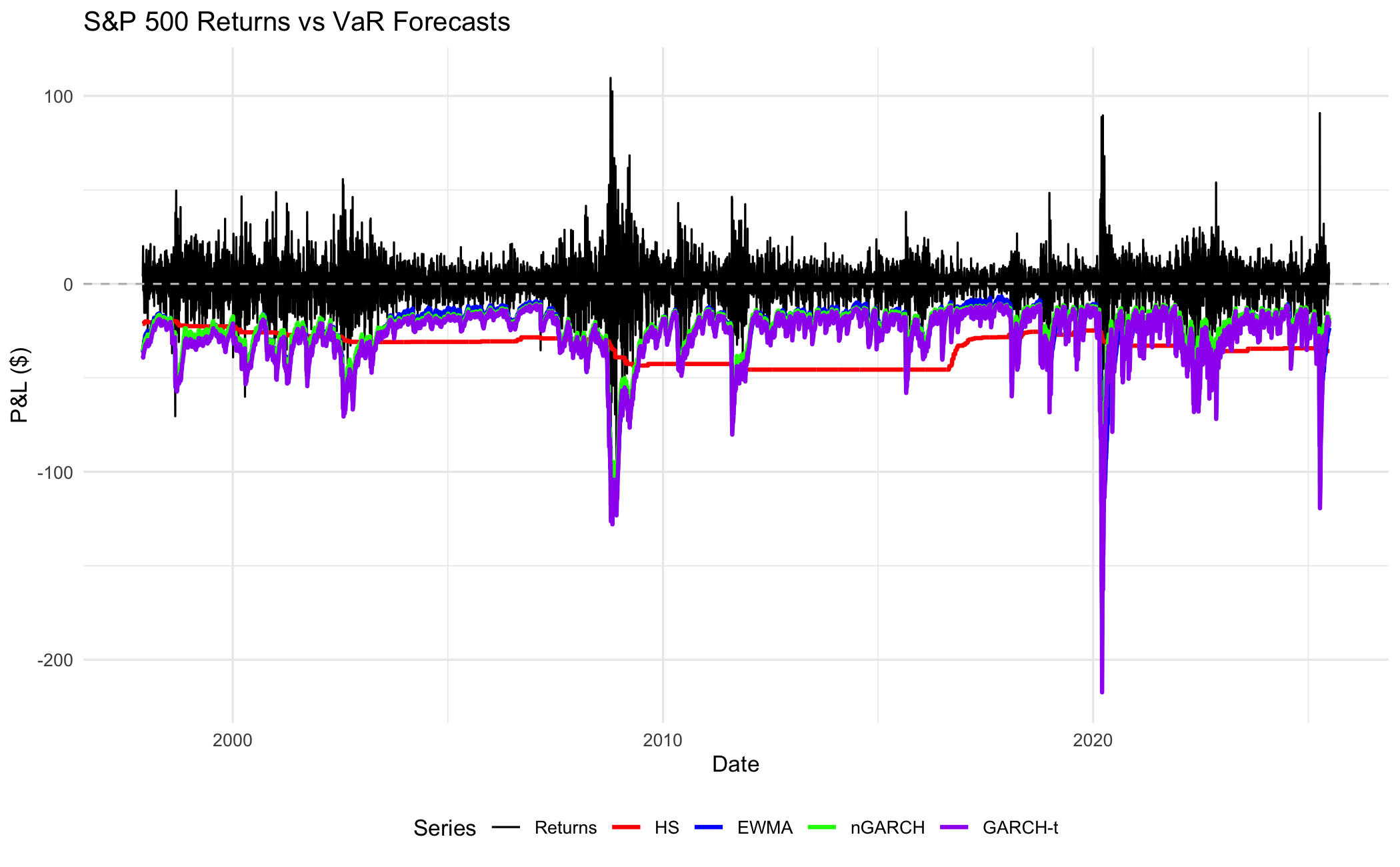
The backtest data frame contains VaR and ES forecasts for all methods, along with actual returns and dates. We can visualise the forecasts against actual returns to see how well our models capture market risk.
27.4 Violations
A violation occurs when the realised return reaches or falls below the negative of the VaR forecast, \(\CompoundReturns_t \leq -\VaR_t\). For a well-calibrated VaR model, violations should occur at the expected frequency — a r round(par$probability*100, 1)% VaR model should be exceeded roughly r round(par$probability*100, 1)% of the time.
We compute violation indicators by comparing actual losses to the VaR forecasts. The violation ratio scales the outcome by what the model predicted:
\[\ViolRatio = \frac{\ExceptionCount_1}{\probability \TestWindow}\]
where \(\ExceptionCount_1\) is the number of violations and \(\TestWindow\) the length of the testing window. A ratio of one is the ideal. Above one the model forecasts too little risk, below one too much.
VaR_methods = c("VaR.HS", "VaR.EWMA", "VaR.nGARCH", "VaR.tGARCH")
PL = backtest$y * par$value

Violations_r = matrix(0, nrow = nrow(backtest), ncol = length(VaR_methods))
colnames(Violations_r) = VaR_methods

for (i in 1:length(VaR_methods)) {
    VaR_values = backtest[, VaR_methods[i]]
    Violations_r[, i] = ifelse(PL <= -VaR_values, 1, 0)
}

violation_counts_r = colSums(Violations_r)
violation_rates_r = violation_counts_r / nrow(Violations_r)
violation_ratios_r = violation_rates_r / par$probability

short_names = c("HS", "EWMA", "nGARCH", "GARCH-t")
cat("Violation counts:\n")
for (i in seq_along(short_names)) {
    cat(sprintf("  %-8s: %d\n", short_names[i], violation_counts_r[i]))
}
cat("\nViolation rates:\n")
for (i in seq_along(short_names)) {
    cat(sprintf("  %-8s: %.2f%%\n", short_names[i], violation_rates_r[i] * 100))
}
cat("\nViolation ratios:\n")
for (i in seq_along(short_names)) {
    cat(sprintf("  %-8s: %.2f\n", short_names[i], violation_ratios_r[i]))
}
cat(sprintf("\nExpected rate: %d%%\n", as.integer(par$probability * 100)))
Violation counts:
HS : 107
EWMA : 153
nGARCH : 136
GARCH-t : 87
Violation rates:
HS : 1.54%
EWMA : 2.21%
nGARCH : 1.96%
GARCH-t : 1.25%
Violation ratios:
HS : 1.54
EWMA : 2.21
nGARCH : 1.96
GARCH-t : 1.25
Expected rate: 1%VaR_methods_py = ['VaR.HS', 'VaR.EWMA', 'VaR.nGARCH', 'VaR.tGARCH']
PL_py = backtest['y'].values * par['value']
Violations_py = np.zeros((len(backtest), len(VaR_methods_py)))
for i, method in enumerate(VaR_methods_py):
VaR_values = backtest[method].values
Violations_py[:, i] = (PL_py <= -VaR_values).astype(int)
violation_counts_py = Violations_py.sum(axis=0)
violation_rates_py = violation_counts_py / len(Violations_py)
violation_ratios_py = violation_rates_py / par['probability']
short_names_py = ['HS', 'EWMA', 'nGARCH', 'GARCH-t']
print("Violation counts:")
for i, name in enumerate(short_names_py):
print(f" {name:<8s}: {int(violation_counts_py[i])}")
print(f"\nViolation rates:")
for i, name in enumerate(short_names_py):
print(f" {name:<8s}: {violation_rates_py[i]*100:.2f}%")
print(f"\nViolation ratios:")
for i, name in enumerate(short_names_py):
print(f" {name:<8s}: {violation_ratios_py[i]:.2f}")
print(f"\nExpected rate: {int(par['probability']*100)}%")Violation counts:
HS : 107
EWMA : 153
nGARCH : 136
GARCH-t : 87
Violation rates:
HS : 1.54%
EWMA : 2.21%
nGARCH : 1.96%
GARCH-t : 1.25%
Violation ratios:
HS : 1.54
EWMA : 2.21
nGARCH : 1.96
GARCH-t : 1.25
Expected rate: 1%VaR_methods_jl = ["VaR.HS", "VaR.EWMA", "VaR.nGARCH", "VaR.tGARCH"];
method_names_jl = ["HS", "EWMA", "nGARCH", "GARCH-t"];
PL_jl = backtest[!, :y] .* par["value"];
n_obs = nrow(backtest);
Violations_jl = zeros(Int, n_obs, length(VaR_methods_jl));
for (i, method) in enumerate(VaR_methods_jl)
VaR_values = backtest[!, Symbol(method)]
Violations_jl[:, i] = Int.(PL_jl .<= -VaR_values)
end
violation_counts_jl = vec(sum(Violations_jl, dims=1));
violation_rates_jl = violation_counts_jl ./ n_obs;
violation_ratios_jl = violation_rates_jl ./ par["probability"];
using Printf
println("Violation counts:");
for (i, method) in enumerate(method_names_jl)
@printf(" %-8s: %d\n", method, violation_counts_jl[i])
end
println("\nViolation rates:");
for (i, method) in enumerate(method_names_jl)
@printf(" %-8s: %.2f%%\n", method, violation_rates_jl[i]*100)
end
println("\nViolation ratios:");
for (i, method) in enumerate(method_names_jl)
@printf(" %-8s: %.2f\n", method, violation_ratios_jl[i])
end
@printf("\nExpected rate: %d%%\n", Int(par["probability"]*100))Violation counts:
HS : 107
EWMA : 153
nGARCH : 136
GARCH-t : 87
Violation rates:
HS : 1.54%
EWMA : 2.21%
nGARCH : 1.96%
GARCH-t : 1.25%
Violation ratios:
HS : 1.54
EWMA : 2.21
nGARCH : 1.96
GARCH-t : 1.25
Expected rate: 1%27.5 Violation patterns over time
The timing of violations tells us whether a model adapts to changing market conditions.
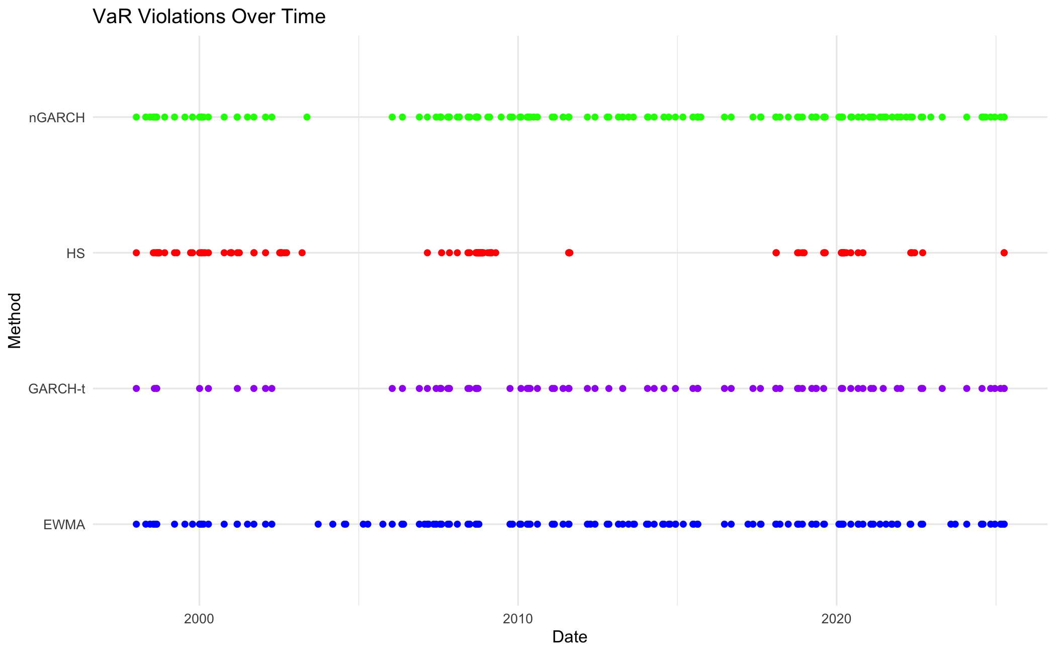
The violations cluster visibly around early 2020, at the onset of the Covid-19 market disruption. The clustering is pronounced for all four methods, with violations arriving in concentrated bursts rather than singly.
27.6 Statistical analysis of VaR
The violation analysis reveals differences between methods. However, we cannot conclude from violation counts alone whether these differences represent genuine model failures or acceptable random variation.
A model with more violations is not necessarily wrong. Sampling variation can produce that difference.
We implement the testing framework developed by Christoffersen (1998). This framework tests two properties that well-functioning VaR models must satisfy.
27.6.1 Coverage test
The Bernoulli coverage test examines whether the violation rate is statistically different from the expected rate.
Violations are iid Bernoulli under \(H_0\). Let \(\ExceptionCount_0\) and \(\ExceptionCount_1\) be the counts of non-violation and violation days in the \(\TestWindow\)-day testing window. The restricted likelihood fixes the violation probability at the nominal \(\probability\). The unrestricted likelihood instead uses the estimated rate \(\hat\probability = \ExceptionCount_1 / \TestWindow\):
\[\lik(\probability) = (1-\probability)^{\ExceptionCount_0}\probability^{\ExceptionCount_1}, \qquad \lik(\hat\probability) = (1-\hat\probability)^{\ExceptionCount_0}\hat\probability^{\ExceptionCount_1}\]
The likelihood ratio statistic
\[\text{LR}_{uc} = -2\left(\log \lik(\probability) - \log \lik(\hat\probability)\right)\]
is asymptotically \(\chi^2_{(1)}\) under \(H_0\).
Asymptotically is the operative word, and the approximation is weakest exactly where regulatory backtesting lives. At \(\probability = 0.01\) over a 250-day year the expected number of violations is 2.5, and a test whose reference distribution assumes a large sample is being asked to rule on a handful of events.
The zero-violation case shows how far apart the calibrations can be. With \(\ExceptionCount_1 = 0\) the statistic collapses to \(2\TestWindow\log[1/(1-\probability)]\), which at \(\probability = 0.01\) and \(\TestWindow = 250\) is about 5.03. Read against \(\chi^2_{(1)}\) that gives a p-value of 0.025 and rejects at 5%. But a correctly calibrated model produces no violations at all with probability \(0.99^{250} \approx 8.1\%\), which is not a rare event, so the rejection should be suspect.
Working the same statistic out exactly under the binomial gives a different answer, and how much different depends on a choice the asymptotic version hides. A two-sided test on a discrete, asymmetric distribution has to decide which outcomes count as “at least as extreme”, and the usual conventions do not agree:
| Convention | p-value |
|---|---|
| Asymptotic \(\chi^2_{(1)}\) | 0.025 |
| Exact, ordered by the likelihood-ratio statistic | 0.095 |
| Exact, doubling the lower-tail probability | 0.162 |
Exact, ordered by density (R’s binom.test) |
0.189 |
Only the first rejects at 5%, and it is the one whose assumptions are least defensible here. The three exact conventions span a factor of two among themselves, which matters before quoting any of them to three decimal places. Seeing no violations in a year is consistent with a model that is too conservative, but 250 observations cannot establish it.
Two things follow. State which convention produced a reported p-value, since on short windows the choice can decide the verdict, and be wary of the \(\chi^2\) result there at all. Our own testing window here is r format(par$WT, big.mark = ",") observations, far longer than the 250-day regulatory case, so the asymptotic reference is on much firmer ground for the results below. The caution matters when reusing these functions on a one-year window.
# Bernoulli coverage test (from Financial Risk Forecasting book)
# Convention: a log-likelihood term with count 0 contributes 0
bern_test = function(p, v) {
    lv = length(v)
    sv = sum(v)
    al = 0
    if (lv - sv > 0) al = al + log(1-p) * (lv-sv)
    if (sv > 0) al = al + log(p) * sv
    ph = sv / lv
    bl = 0
    if (lv - sv > 0) bl = bl + log(1-ph) * (lv-sv)
    if (sv > 0) bl = bl + log(ph) * sv
    return(-2 * (al-bl))
}
def bern_test(p, v):
"""Bernoulli coverage test. Convention: a log-likelihood term with count 0 contributes 0"""
lv = len(v)
sv = np.sum(v)
al = 0.0
if lv - sv > 0:
al += np.log(1-p) * (lv-sv)
if sv > 0:
al += np.log(p) * sv
ph = sv / lv
bl = 0.0
if lv - sv > 0:
bl += np.log(1-ph) * (lv-sv)
if sv > 0:
bl += np.log(ph) * sv
return -2 * (al - bl)# Convention: a log-likelihood term with count 0 contributes 0
function bern_test(p, v)
lv = length(v)
sv = sum(v)
al = 0.0
if lv - sv > 0
al += log(1-p) * (lv-sv)
end
if sv > 0
al += log(p) * sv
end
ph = sv / lv
bl = 0.0
if lv - sv > 0
bl += log(1-ph) * (lv-sv)
end
if sv > 0
bl += log(ph) * sv
end
return -2 * (al - bl)
end;Bernoulli Coverage Test Results:
H0: Violation rate equals expected rate
m = c("HS", "EWMA", "nGARCH", "GARCH-t")

for (i in 1:4) {
    test_stat = bern_test(par$probability, Violations_r[, i])
    p_value = 1 - pchisq(test_stat, df = 1)
    result = ifelse(p_value < 0.05, "REJECT", "PASS")
    cat(sprintf("%-8s: Test statistic = %.3f, p-value = %.4f (%s)\n",
                m[i], test_stat, p_value, result))
}
HS : Test statistic = 17.678, p-value = 0.0000 (REJECT)
EWMA : Test statistic = 75.779, p-value = 0.0000 (REJECT)
nGARCH : Test statistic = 50.480, p-value = 0.0000 (REJECT)
GARCH-t : Test statistic = 4.183, p-value = 0.0408 (REJECT)m_py = ['HS', 'EWMA', 'nGARCH', 'GARCH-t']
for i in range(4):
test_stat = bern_test(par['probability'], Violations_py[:, i])
p_value = 1 - stats.chi2.cdf(test_stat, df=1)
result = "REJECT" if p_value < 0.05 else "PASS"
print(f"{m_py[i]:<8s}: Test statistic = {test_stat:.3f}, p-value = {p_value:.4f} ({result})")HS : Test statistic = 17.678, p-value = 0.0000 (REJECT)
EWMA : Test statistic = 75.779, p-value = 0.0000 (REJECT)
nGARCH : Test statistic = 50.480, p-value = 0.0000 (REJECT)
GARCH-t : Test statistic = 4.183, p-value = 0.0408 (REJECT)using Printf, Distributions
m_jl = ["HS", "EWMA", "nGARCH", "GARCH-t"];
for i in 1:4
test_stat = bern_test(par["probability"], Violations_jl[:, i])
p_value = 1 - cdf(Chisq(1), test_stat)
result = p_value < 0.05 ? "REJECT" : "PASS"
@printf("%-8s: Test statistic = %.3f, p-value = %.4f (%s)\n", m_jl[i], test_stat, p_value, result)
endHS : Test statistic = 17.678, p-value = 0.0000 (REJECT)
EWMA : Test statistic = 75.779, p-value = 0.0000 (REJECT)
nGARCH : Test statistic = 50.480, p-value = 0.0000 (REJECT)
GARCH-t : Test statistic = 4.183, p-value = 0.0408 (REJECT)27.6.2 Independence test
The independence test examines whether violations arrive randomly over time or cluster together. Clustering indicates that the model reacts too slowly to volatility changes, allowing repeated surprises during stress periods.
We model violations as a first-order Markov chain where today’s violation probability depends only on yesterday’s outcome. Under the null hypothesis of independence, the probability of a violation today should be the same regardless of whether there was a violation yesterday.
Let \(\ExceptionCount_{ij}\) be the count of transitions from state \(i\) (yesterday) to state \(j\) (today), and \(\TransProb_{ij}\) the corresponding transition probability. Under \(H_0\), tomorrow’s violation probability does not depend on today’s state, so the restricted model estimates a single pooled rate rather than fixing it at the nominal \(\probability\), which the coverage test above already checks separately. The unrestricted model instead estimates the two transition probabilities separately:
\[\hat\TransProb_2 = \frac{\ExceptionCount_{01}+\ExceptionCount_{11}}{\ExceptionCount_{00}+\ExceptionCount_{01}+\ExceptionCount_{10}+\ExceptionCount_{11}}, \qquad \hat\TransProb_{01} = \frac{\ExceptionCount_{01}}{\ExceptionCount_{00}+\ExceptionCount_{01}}, \qquad \hat\TransProb_{11} = \frac{\ExceptionCount_{11}}{\ExceptionCount_{10}+\ExceptionCount_{11}}\]
\[\lik(\hat\TransProb_2) = (1-\hat\TransProb_2)^{\ExceptionCount_{00}+\ExceptionCount_{10}}\,\hat\TransProb_2^{\ExceptionCount_{01}+\ExceptionCount_{11}}\]
\[\lik(\hat\TransProb_{01},\hat\TransProb_{11}) = (1-\hat\TransProb_{01})^{\ExceptionCount_{00}}\,\hat\TransProb_{01}^{\ExceptionCount_{01}}\,(1-\hat\TransProb_{11})^{\ExceptionCount_{10}}\,\hat\TransProb_{11}^{\ExceptionCount_{11}}\]
The likelihood ratio statistic
\[\text{LR}_{ind} = -2\left(\log \lik(\hat\TransProb_2) - \log \lik(\hat\TransProb_{01}, \hat\TransProb_{11})\right)\]
is asymptotically \(\chi^2_{(1)}\) under \(H_0\).
# Independence test function (from Financial Risk Forecasting book)
# Convention: a log-likelihood term with count 0 contributes 0. A transition
# probability is only ever computed inside a term whose count is positive, so
# a zero denominator (e.g. V_10 = V_11 = 0) never gets formed.
ind_test = function(V) {
    n = length(V)
    if (sum(V) == 0 || sum(V) == n) return(NA)

    V_00 = 0; V_01 = 0; V_10 = 0; V_11 = 0
    for (i in 2:n) {
        if (V[i-1] == 0 && V[i] == 0) V_00 = V_00 + 1
        else if (V[i-1] == 0 && V[i] == 1) V_01 = V_01 + 1
        else if (V[i-1] == 1 && V[i] == 0) V_10 = V_10 + 1
        else if (V[i-1] == 1 && V[i] == 1) V_11 = V_11 + 1
    }

    hat_p = (V_01 + V_11) / (V_00 + V_01 + V_10 + V_11)
    al = 0
    if (V_00 + V_10 > 0) al = al + log(1 - hat_p) * (V_00 + V_10)
    if (V_01 + V_11 > 0) al = al + log(hat_p) * (V_01 + V_11)

    bl = 0
    if (V_00 > 0) { p_01 = V_01 / (V_00 + V_01); bl = bl + log(1 - p_01) * V_00 }
    if (V_01 > 0) { p_01 = V_01 / (V_00 + V_01); bl = bl + log(p_01) * V_01 }
    if (V_10 > 0) { p_11 = V_11 / (V_10 + V_11); bl = bl + log(1 - p_11) * V_10 }
    if (V_11 > 0) { p_11 = V_11 / (V_10 + V_11); bl = bl + log(p_11) * V_11 }

    return(-2 * (al - bl))
}
def ind_test(V):
"""Independence test for violation clustering.
Convention: a log-likelihood term with count 0 contributes 0. A transition
probability is only ever computed inside a term whose count is positive, so
a zero denominator (e.g. V_10 = V_11 = 0) never gets formed."""
n = len(V)
if np.sum(V) == 0 or np.sum(V) == n:
return float('nan')
V_00 = V_01 = V_10 = V_11 = 0
for i in range(1, n):
if V[i-1] == 0 and V[i] == 0:
V_00 += 1
elif V[i-1] == 0 and V[i] == 1:
V_01 += 1
elif V[i-1] == 1 and V[i] == 0:
V_10 += 1
elif V[i-1] == 1 and V[i] == 1:
V_11 += 1
hat_p = (V_01 + V_11) / (V_00 + V_01 + V_10 + V_11)
al = 0.0
if V_00 + V_10 > 0:
al += np.log(1 - hat_p) * (V_00 + V_10)
if V_01 + V_11 > 0:
al += np.log(hat_p) * (V_01 + V_11)
bl = 0.0
if V_00 > 0:
p_01 = V_01 / (V_00 + V_01)
bl += np.log(1 - p_01) * V_00
if V_01 > 0:
p_01 = V_01 / (V_00 + V_01)
bl += np.log(p_01) * V_01
if V_10 > 0:
p_11 = V_11 / (V_10 + V_11)
bl += np.log(1 - p_11) * V_10
if V_11 > 0:
p_11 = V_11 / (V_10 + V_11)
bl += np.log(p_11) * V_11
return -2 * (al - bl)# Convention: a log-likelihood term with count 0 contributes 0. A transition
# probability is only ever computed inside a term whose count is positive, so
# a zero denominator (e.g. V_10 = V_11 = 0) never gets formed.
function ind_test(V)
n = length(V)
if sum(V) == 0 || sum(V) == n
return NaN
end
V_00 = V_01 = V_10 = V_11 = 0
for i in 2:n
if V[i-1] == 0 && V[i] == 0
V_00 += 1
elseif V[i-1] == 0 && V[i] == 1
V_01 += 1
elseif V[i-1] == 1 && V[i] == 0
V_10 += 1
elseif V[i-1] == 1 && V[i] == 1
V_11 += 1
end
end
hat_p = (V_01 + V_11) / (V_00 + V_01 + V_10 + V_11)
al = 0.0
if V_00 + V_10 > 0
al += log(1 - hat_p) * (V_00 + V_10)
end
if V_01 + V_11 > 0
al += log(hat_p) * (V_01 + V_11)
end
bl = 0.0
if V_00 > 0
p_01 = V_01 / (V_00 + V_01)
bl += log(1 - p_01) * V_00
end
if V_01 > 0
p_01 = V_01 / (V_00 + V_01)
bl += log(p_01) * V_01
end
if V_10 > 0
p_11 = V_11 / (V_10 + V_11)
bl += log(1 - p_11) * V_10
end
if V_11 > 0
p_11 = V_11 / (V_10 + V_11)
bl += log(p_11) * V_11
end
return -2 * (al - bl)
end;Independence Test Results:
H0: Violations are independent over time
for (i in 1:4) {
    test_stat = ind_test(Violations_r[, i])
    p_value = 1 - pchisq(test_stat, df = 1)
    result = ifelse(is.na(p_value), "UNDEFINED", ifelse(p_value < 0.05, "REJECT", "PASS"))
    cat(sprintf("%-8s: Test statistic = %.3f, p-value = %.4f (%s)\n",
                m[i], test_stat, p_value, result))
}
HS : Test statistic = 13.343, p-value = 0.0003 (REJECT)
EWMA : Test statistic = 3.143, p-value = 0.0762 (PASS)
nGARCH : Test statistic = 1.703, p-value = 0.1919 (PASS)
GARCH-t : Test statistic = 4.776, p-value = 0.0289 (REJECT)for i in range(4):
test_stat = ind_test(Violations_py[:, i])
p_value = 1 - stats.chi2.cdf(test_stat, df=1)
if np.isnan(test_stat):
result = "UNDEFINED"
else:
result = "REJECT" if p_value < 0.05 else "PASS"
print(f"{m_py[i]:<8s}: Test statistic = {test_stat:.3f}, p-value = {p_value:.4f} ({result})")HS : Test statistic = 13.343, p-value = 0.0003 (REJECT)
EWMA : Test statistic = 3.143, p-value = 0.0762 (PASS)
nGARCH : Test statistic = 1.703, p-value = 0.1919 (PASS)
GARCH-t : Test statistic = 4.776, p-value = 0.0289 (REJECT)using Printf, Distributions
for i in 1:4
test_stat = ind_test(Violations_jl[:, i])
p_value = isnan(test_stat) ? NaN : 1 - cdf(Chisq(1), test_stat)
result = isnan(test_stat) ? "UNDEFINED" : (p_value < 0.05 ? "REJECT" : "PASS")
@printf("%-8s: Test statistic = %.3f, p-value = %.4f (%s)\n", m_jl[i], test_stat, p_value, result)
endHS : Test statistic = 13.343, p-value = 0.0003 (REJECT)
EWMA : Test statistic = 3.143, p-value = 0.0762 (PASS)
nGARCH : Test statistic = 1.703, p-value = 0.1919 (PASS)
GARCH-t : Test statistic = 4.776, p-value = 0.0289 (REJECT)Where the independence test rejects, it confirms the clustering seen in the violation plot, with violations in those series arriving in runs rather than one at a time.
27.7 ES backtesting
ES measures the average loss in the worst cases beyond the VaR threshold:
\[\ES(\probability) = -\E[\CompoundReturns_t \mid \CompoundReturns_t \leq -\VaR(\probability)]\]
This definition applies to continuous return distributions. In general, ES is the average of all quantiles beyond \(\probability\).
Unlike VaR, ES cannot be backtested by counting violations, for two reasons:
- ES is not defined by a single threshold breach but depends on the full shape of the loss tail
- ES is sensitive to rare, extreme losses that occur infrequently
ES is also not elicitable on its own, though Fissler and Ziegel (2016) showed that the pair \((\VaR, \ES)\) is jointly elicitable. Elicitability governs how competing forecasts are ranked, not whether a measure can be backtested, and Section 27.10.1 returns to the distinction. ES can be backtested, as the next section shows.
27.7.1 The Acerbi-Székely approach
ES can be backtested with the minimally biased statistic proposed by Acerbi and Székely (2019). The daily score is
\[Z_{\mathrm{ES},t} = \ES_t - \VaR_t - \frac{1}{\probability}\left(-\PortfolioValue\CompoundReturns_t - \VaR_t\right)_+\]
where:
- \(\ES_t\) = ES forecast for day \(t\) (positive loss magnitude, in the same units as P&L)
- \(\VaR_t\) = VaR forecast for day \(t\) (positive loss magnitude, in the same units as P&L)
- \(\PortfolioValue\CompoundReturns_t\) = realised P&L for day \(t\), the portfolio value times the realised return (negative for losses)
- \(\probability\) = tail probability (e.g., 0.01 for 1% VaR, corresponding to a 99% confidence level)
- \((x)_+ = \max(x, 0)\) is the positive part function, so the term is non-zero only when the loss exceeds VaR
The score \(Z_{\mathrm{ES},t}\) is computed for every day in the testing window, not only on violation days. On days without a VaR breach, \((-\PortfolioValue\CompoundReturns_t - \VaR_t)_+ = 0\) and the score reduces to \(\ES_t - \VaR_t > 0\). We summarise the window by the sample mean
\[\bar Z_{\mathrm{ES}} = \frac{1}{\TestWindow}\sum_{t=1}^{\TestWindow} Z_{\mathrm{ES},t}\]
and standardise it by \(s_Z\), the empirical standard deviation of the daily scores, which gives the diagnostic
\[\frac{\sqrt{\TestWindow}\,\bar Z_{\mathrm{ES}}}{s_Z}\]
The symbols \(Z_{\mathrm{ES},t}\), \(\bar Z_{\mathrm{ES}}\) and \(s_Z\) are local to this diagnostic section.
We report both quantities descriptively and attach no p-value to either. The distribution of \(\bar Z_{\mathrm{ES}}\) under the null depends on the forecast model that produced the VaR and ES numbers, so there is no universal reference distribution to read a p-value from. A formal test requires simulating the null from each model’s own predictive distribution, which is the Monte Carlo procedure Acerbi and Székely (2019) use.
Note
The standardisation treats the daily scores as independent, which rolling-window forecasts violate. Under positive serial dependence \(s_Z\) understates the dispersion of \(\bar Z_{\mathrm{ES}}\), so the diagnostic is larger in absolute value than the data warrant. It is also symmetric in sign here, although Acerbi and Székely (2019)’s minimally biased version is directed against ES underestimation.
When the ES model is correctly specified, the statistic is unbiased apart from a small prudential bias. That bias disappears when the accompanying VaR forecast is exact.
27.7.2 Implementation
# Minimally biased ES backtest (Acerbi-Székely 2019)
# Computes the daily score Z_ES,t for every day in the testing window
Z_ES = function(ES_t, VaR_t, PL_t, p = 0.01) {
    ES_t - VaR_t - (1 / p) * pmax(0, -PL_t - VaR_t)
}
def Z_ES(ES_t, VaR_t, PL_t, p=0.01):
"""Minimally biased ES backtest score (Acerbi-Székely 2019).
Computes the daily score Z_ES,t for every day in the testing window."""
return ES_t - VaR_t - (1 / p) * np.maximum(0, -PL_t - VaR_t)function Z_ES(ES_t, VaR_t, PL_t; p=0.01)
# Minimally biased ES backtest score (Acerbi-Székely 2019)
# Computes the daily score Z_ES,t for every day in the testing window
return ES_t .- VaR_t .- (1 / p) .* max.(0, .-PL_t .- VaR_t)
end;27.7.3 ES test results
We compute \(Z_{\mathrm{ES},t}\) for every day in the testing window and report \(\bar Z_{\mathrm{ES}}\) alongside its standardised counterpart.
Note
The ES statistic carries much less information than the VaR coverage tests. Non-violation days contribute \(\ES_t - \VaR_t\) to the score. Only the realised-loss penalty activates on violation days, so few realised tail losses limit what the statistic can reveal. When the number of violations is very small (fewer than about 10), the ES diagnostic should be interpreted with caution.
ES_methods = c("ES.HS", "ES.EWMA", "ES.nGARCH", "ES.tGARCH")
es_means_r = numeric(4)
es_std_r = numeric(4)
es_violations_r = integer(4)

for (i in 1:4) {
    var_col = VaR_methods[i]
    es_col = ES_methods[i]

    var_forecasts = backtest[, var_col]
    es_forecasts = backtest[, es_col]

    # Compute daily score over ALL days
    Z_values = Z_ES(es_forecasts, var_forecasts, PL, p = par$probability)

    n = length(Z_values)
    mean_Z = mean(Z_values)
    s_Z = sd(Z_values)
    standardised = sqrt(n) * mean_Z / s_Z
    n_violations = sum(PL <= -var_forecasts)

    es_means_r[i] = mean_Z
    es_std_r[i] = standardised
    es_violations_r[i] = n_violations
    cat(sprintf("%-8s: mean score = %.4f, standardised = %.3f, violations = %d\n",
                m[i], mean_Z, standardised, n_violations))
}
HS : mean score = -7.5290, standardised = -2.362, violations = 107
EWMA : mean score = -12.0302, standardised = -6.334, violations = 153
nGARCH : mean score = -9.0951, standardised = -5.306, violations = 136
GARCH-t : mean score = -1.5244, standardised = -1.051, violations = 87ES_methods_py = ['ES.HS', 'ES.EWMA', 'ES.nGARCH', 'ES.tGARCH']
es_results_py = []
for i in range(4):
var_col = VaR_methods_py[i]
es_col = ES_methods_py[i]
var_forecasts = backtest[var_col].values
es_forecasts = backtest[es_col].values
# Compute daily score over ALL days
Z_values = Z_ES(es_forecasts, var_forecasts, PL_py, p=par['probability'])
n = len(Z_values)
mean_Z = np.mean(Z_values)
s_Z = np.std(Z_values, ddof=1)
standardised = np.sqrt(n) * mean_Z / s_Z
n_violations = int(np.sum(PL_py <= -var_forecasts))
es_results_py.append({
'Method': m_py[i],
'Mean_Score': round(mean_Z, 4),
'Standardised': round(standardised, 3),
'Violations': n_violations
})
print(f"{m_py[i]:<8s}: mean score = {mean_Z:.4f}, standardised = {standardised:.3f}, violations = {n_violations}")HS : mean score = -7.5290, standardised = -2.362, violations = 107
EWMA : mean score = -12.0302, standardised = -6.334, violations = 153
nGARCH : mean score = -9.0951, standardised = -5.306, violations = 136
GARCH-t : mean score = -1.5244, standardised = -1.051, violations = 87using Printf, Statistics
ES_methods_jl = ["ES.HS", "ES.EWMA", "ES.nGARCH", "ES.tGARCH"];
es_means_jl = zeros(4);
es_std_jl = zeros(4);
es_violations_jl = zeros(Int, 4);
for i in 1:4
var_col = Symbol(VaR_methods_jl[i])
es_col = Symbol(ES_methods_jl[i])
var_forecasts = backtest[!, var_col]
es_forecasts = backtest[!, es_col]
# Compute daily score over ALL days
Z_values = Z_ES(es_forecasts, var_forecasts, PL_jl, p=par["probability"])
n = length(Z_values)
mean_Z = mean(Z_values)
s_Z = std(Z_values)
standardised = sqrt(n) * mean_Z / s_Z
n_violations = sum(PL_jl .<= -var_forecasts)
es_means_jl[i] = mean_Z
es_std_jl[i] = standardised
es_violations_jl[i] = n_violations
@printf("%-8s: mean score = %.4f, standardised = %.3f, violations = %d\n", m_jl[i], mean_Z, standardised, n_violations)
endHS : mean score = -7.5290, standardised = -2.362, violations = 107
EWMA : mean score = -12.0302, standardised = -6.334, violations = 153
nGARCH : mean score = -9.0951, standardised = -5.306, violations = 136
GARCH-t : mean score = -1.5244, standardised = -1.051, violations = 8727.7.4 ES test comparison
   Method   Mean_R Mean_Python Mean_Julia  Std_R Std_Python Std_Julia
1      HS  -7.5290     -7.5290    -7.5290 -2.362     -2.362    -2.362
2    EWMA -12.0302    -12.0302   -12.0302 -6.334     -6.334    -6.334
3  nGARCH  -9.0951     -9.0951    -9.0951 -5.306     -5.306    -5.306
4 GARCH-t  -1.5244     -1.5244    -1.5244 -1.051     -1.051    -1.051
27.7.5 Interpretation
- A negative \(\bar Z_{\mathrm{ES}}\) indicates ES underestimation (losses exceed forecasts)
- A positive value indicates overestimation (forecasts are too conservative)
- Values close to zero imply consistency between forecasts and realisations
The standardised column expresses the same comparison in units of the dispersion of the daily scores, which makes the four methods comparable with one another. For the reason given above it is a descriptive quantity rather than a test statistic, so read its sign and its size relative to the other methods, not a significance level.
A relative variant divides \(Z_{\mathrm{ES},t}\) by \(\ES_t\). That gives a scale-free adjustment factor, which is useful when regulators scale capital multipliers.
27.8 Beyond the three tests
That completes the tests we implement. Coverage asks whether the model breaches at the right rate, independence whether the breaches arrive in the right pattern, and the ES diagnostic whether the losses beyond the threshold were the right size. A model that passes all three has answered every question we have put to it.
The rest of the chapter puts different questions. The next section asks what the whole predictive distribution looks like rather than one point of it, and is implemented like the tests above. The section after that asks how two models should be ranked against each other, and is theoretical background rather than code — it supplies the machinery the comparison chapters use.
27.9 Testing the whole distribution: the PIT
Every test so far looks at one point of the forecast distribution. The coverage and independence tests use the violation indicator at \(\probability\), and the ES diagnostic uses the tail beyond it. A model can get that one point right and be wrong everywhere else, and none of these tests would notice.
The probability integral transform tests the whole thing. If \(\CDF_t\) is the model’s predictive distribution for day \(t\), formed using only information available beforehand, then
\[u_t = \CDF_t(\CompoundReturns_t)\]
should be uniform on \([0,1]\) when the model is right, and independent across days. The intuition is that \(\CDF_t\) tells us what fraction of the forecast distribution lies below each outcome. If the forecasts are correct, the outcomes land uniformly through them. The result is usually attributed to Rosenblatt (1952).
Uniformity is easier to read after mapping back to a normal scale, \(\NormalQuantile(u_t)\), which should be standard normal. Both forms carry the same information, and the histogram of \(u_t\) is the more direct diagnostic. A hump in the middle means the predictive distribution is too wide, since outcomes keep landing near its centre, and mass piling up at both ends means it is too narrow.
The forecasts we backtested were produced by rolling one-day models, so we can form the PIT for each. Under the normal methods the predictive distribution is normal with the forecast volatility. The volatility that produced each VaR can be recovered from that VaR by inverting the same formula.
# Recover the forecast volatility from each VaR, then form the PIT.
# VaR = -qnorm(p) * sigma * value, so sigma = VaR / (-qnorm(p) * value)
pit_methods = c("EWMA", "nGARCH")
u = list()
for (m in pit_methods) {
    sigma_hat = backtest[[paste0("VaR.", m)]] / (-qnorm(par$probability) * par$value)
    u[[m]] = pnorm(backtest$y, mean = 0, sd = sigma_hat)
}

for (m in pit_methods) {
    ks = ks.test(u[[m]], "punif")
    cat(sprintf("%-8s mean %.3f (0.5)  sd %.3f (0.289)  KS p = %.4f\n",
        m, mean(u[[m]]), sd(u[[m]]), ks$p.value))
}
Warning messages:
1: In ks.test.default(u[[m]], "punif") :
ties should not be present for the one-sample Kolmogorov-Smirnov test
2: In ks.test.default(u[[m]], "punif") :
ties should not be present for the one-sample Kolmogorov-Smirnov testEWMA mean 0.517 (0.5) sd 0.280 (0.289) KS p = 0.0000
nGARCH mean 0.516 (0.5) sd 0.276 (0.289) KS p = 0.0000pit_methods = ['EWMA', 'nGARCH']
u = {}
for m in pit_methods:
sigma_hat = backtest[f'VaR.{m}'].values / (-stats.norm.ppf(par['probability']) * par['value'])
u[m] = stats.norm.cdf(backtest['y'].values, loc=0, scale=sigma_hat)
for m in pit_methods:
ks = stats.kstest(u[m], 'uniform')
print(f"{m:<8} mean {np.mean(u[m]):.3f} (0.5) sd {np.std(u[m], ddof=1):.3f} (0.289) KS p = {ks.pvalue:.4f}")EWMA mean 0.517 (0.5) sd 0.280 (0.289) KS p = 0.0000
nGARCH mean 0.516 (0.5) sd 0.276 (0.289) KS p = 0.0000using HypothesisTests
pit_methods = ["EWMA", "nGARCH"]
u_jl = Dict{String, Vector{Float64}}()
for m in pit_methods
sigma_hat = backtest[!, "VaR.$m"] ./ (-quantile(Normal(), par["probability"]) * par["value"])
u_jl[m] = cdf.(Normal.(0, sigma_hat), backtest.y)
end
for m in pit_methods
ks = ExactOneSampleKSTest(u_jl[m], Uniform())
@printf("%-8s mean %.3f (0.5) sd %.3f (0.289) KS p = %.4f\n",
m, mean(u_jl[m]), std(u_jl[m]), pvalue(ks))
endEWMA mean 0.517 (0.5) sd 0.280 (0.289) KS p = 0.0000
nGARCH mean 0.516 (0.5) sd 0.276 (0.289) KS p = 0.0000The dashed line is the uniform density a correctly specified model would produce. Departures from it are informative in a way the exception count is not. They show where in the distribution the model is wrong, not merely that it failed at one quantile.
Two cautions. The transform assumes a continuous predictive distribution, so it does not apply directly to historical simulation, whose predictive distribution is discrete — that is why only the two normal-based methods appear above. And the standard uniformity tests assume the \(u_t\) are independent, which rolling forecasts on overlapping estimation windows do not guarantee. Read a rejection as a signal to look at the histogram, not as a calibrated p-value.
This sits alongside the earlier tests rather than displacing them. Get the whole predictive distribution right and every quantile of it is right too, including the one we report, so a PIT that fails is telling us about a defect that may sit nowhere near \(\probability\) — the model could be mis-shaped in the body while landing the 5% quantile by luck.
The converse is the more uncomfortable one. Almost all of the \(u_t\) come from ordinary days, so a histogram can look convincingly flat while the model is badly wrong in the region we actually charge capital against, simply because too few observations ever land there to disturb the picture.
27.10 Forecast evaluation with scoring rules
Exception tests use only the violation indicator and discard the size of every miss. Scoring rules fix this by penalising each daily forecast against the return that actually arrived. The remainder of the chapter is theoretical background on how forecasts are scored and ranked. It is not implemented in code.
27.10.1 Elicitability
The notion that makes scoring rules work is elicitability. A risk measure is elicitable if there exists a scoring function whose expected value is minimised when the forecaster reports the true value. Put differently, an elicitable measure has a consistent scoring function, and any misreport increases the expected score, so a rational forecaster has no incentive to deviate from the truth.
\(\VaR\) is elicitable. On each day the forecaster issues a quantile forecast and we observe the realised return \(\CompoundReturns_t\). Whether a violation occurred is directly observable — either \(\CompoundReturns_t\) fell to or below the forecast or it did not — and this gives us enough information to construct a scoring function whose expected value is uniquely minimised at the true quantile.
\(\ES\) is not elicitable on its own. The difficulty is that on non-violation days there is no single observable event against which to compare the \(\ES\) forecast. \(\ES\) is the conditional expectation of the loss given that it exceeds \(\VaR\), but on a day without a violation we learn nothing about that conditional tail. No scoring function of the pair \((\ES_t, \CompoundReturns_t)\) alone has an expected value minimised at the true \(\ES\).
This asymmetry between \(\VaR\) and \(\ES\) has practical consequences. We can score \(\VaR\) forecasts directly, but \(\ES\) requires a different approach.
27.10.2 VaR scoring via quantile loss
Because \(\VaR\) is elicitable, we can evaluate \(\VaR\) forecasts using the quantile score (also called the tick loss or pinball loss):
\[\QuantileScore_\probability(\Quantile, \CompoundReturns) = (\CompoundReturns - \Quantile)(\probability - \Indicator_{\CompoundReturns \leq \Quantile})\]
where \(\Quantile\) is the forecast quantile (the negative of the \(\VaR\) forecast, on the return scale), \(\CompoundReturns\) is the realised return, and \(\probability\) is the probability level.
The asymmetry in the penalty is the defining feature. When \(\CompoundReturns \leq \Quantile\), a violation has occurred and the loss is weighted by \(1 - \probability\). When \(\CompoundReturns > \Quantile\), the loss is weighted by \(\probability\). For a 1% \(\VaR\) forecast (\(\probability = 0.01\)), violations are penalised 99 times more heavily than non-violations. This asymmetric weighting ensures that the expected score is minimised when \(\Quantile\) equals the true \(\probability\)-quantile of the return distribution.
To compare two models, compute the average quantile score across the backtest window for each and prefer the model with the lower average. Unlike exception tests, the quantile score responds to the magnitude of forecast errors, not merely their direction. A model that misses \(\VaR\) by a small amount on a handful of days is penalised less than one that misses by a large amount, enabling finer distinctions between competing forecasts.
27.10.3 The ES problem and joint elicitability
The non-elicitability of \(\ES\) does not mean it cannot be evaluated — only that it cannot be evaluated in isolation using a consistent scoring function. The Acerbi-Székely diagnostic above evaluates it all the same, because elicitability governs ranking rather than backtesting.
Fissler and Ziegel (2016) resolved the ranking problem by showing that while \(\ES\) alone is not elicitable, the pair \((\VaR, \ES)\) is jointly elicitable. There exists a scoring function of four arguments — the \(\VaR\) forecast, the \(\ES\) forecast, the realised return and the probability level — whose expected value is minimised when both forecasts equal their true values simultaneously.
The intuition is that \(\VaR\) provides the threshold information that \(\ES\) scoring needs. Once the quantile boundary is pinned down correctly, we can score the conditional tail expectation against realised losses in the tail. The two measures complement each other. \(\VaR\) identifies the boundary and \(\ES\) measures the severity beyond it.
The FZ family of loss functions implements this joint scoring, and applied work picks a convenient member such as the FZ0 loss. It penalises forecast errors in both \(\VaR\) and \(\ES\) simultaneously, and its minimisation property means that misreporting either component increases the expected score. This addresses a gap that exception-based tests cannot fill, since those tests have no mechanism for crediting a model that forecasts \(\ES\) well but produces the same violation count as a competitor.
27.10.4 Comparative forecast evaluation
If two models have different average scores, does that reflect better forecasting or mere noise?
The Diebold-Mariano test (Diebold and Mariano 1995) formalises this comparison. Let \(d_t\) denote the difference in scores between two models on day \(t\). Under the null hypothesis of equal predictive ability, the mean of \(d_t\) is zero. The test statistic is the sample mean of \(d_t\) divided by an estimate of its standard error, and is asymptotically normal. Because score differences are typically serially correlated in time series backtests, an appropriate variance estimator such as Newey-West is required.
When more than two models are under consideration, pairwise Diebold-Mariano tests introduce multiple testing problems. Model confidence sets (Hansen et al. 2011) address this by identifying the subset of models that cannot be distinguished from the best performer at a given confidence level, controlling for the simultaneous comparisons.
Score differences should be interpreted alongside their economic significance. A statistically significant but tiny improvement in average score may not justify the additional complexity of a more sophisticated model.
27.11 What the tests show
The three diagnostics answer different questions. The coverage test asks whether violations arrive at the nominal rate, and the violation ratio measures the same discrepancy without a formal test. The independence test asks whether they arrive in clusters, which coverage cannot detect — a model can deliver exactly the expected number of violations and still concentrate them in a fortnight. The ES diagnostic asks whether the average loss beyond \(\VaR\) matched what the tail delivered, and it stays descriptive because its null distribution depends on the model that produced the forecasts.
A model that survives all three has not been shown to be correct. It has escaped rejection by the tests we have, at the sample size we have.
Acerbi, Carlo, and Balázs Székely. 2019. The Minimally Biased Backtest for Expected Shortfall. Risk.net. https://www.risk.net/cutting-edge/banking/6947266/the-minimally-biased-backtest-for-es.
Christoffersen, Peter F. 1998. “Evaluating Interval Forecasts.” International Economic Review 39 (4): 841–62.
Diebold, Francis X., and Roberto S. Mariano. 1995. “Comparing Predictive Accuracy.” Journal of Business & Economic Statistics 13 (3): 253–63.
Fissler, Tobias, and Johanna F. Ziegel. 2016. “Higher Order Elicitability and Osband’s Principle.” The Annals of Statistics 44 (4): 1680–707. https://doi.org/10.1214/16-AOS1439.
Hansen, Peter R., Asger Lunde, and James M. Nason. 2011. “The Model Confidence Set.” Econometrica 79 (2): 453–97. https://doi.org/10.3982/ECTA5771.
Rosenblatt, Murray. 1952. “Remarks on a Multivariate Transformation.” The Annals of Mathematical Statistics 23 (3): 470–72. https://doi.org/10.1214/aoms/1177729394.