\[ % MathJax has no bm package; redefine \bm in terms of \boldsymbol, which it supports natively \newcommand{\bm}[1]{\boldsymbol{#1}} % --- Operators ----------------------------------------------------------- % Expectation operator \DeclareMathOperator{\E}{E} % Variance operator \DeclareMathOperator{\Var}{Var} % Covariance operator \DeclareMathOperator{\Cov}{Cov} % Correlation operator \DeclareMathOperator{\Corr}{Corr} % Rank operator (Spearman rank correlation) \DeclareMathOperator{\Rank}{Rank} % Skewness operator \DeclareMathOperator{\Skewness}{Skewness} % Kurtosis operator \DeclareMathOperator{\Kurtosis}{Kurtosis} % Difference/differential operator (upright d per ISO 80000-2) \newcommand{\Diff}{\mathrm{d}} % --- Risk Measures ------------------------------------------------------- % Value at Risk \DeclareMathOperator{\VaR}{VaR} % Expected Shortfall \DeclareMathOperator{\ES}{ES} % Marginal Value at Risk \DeclareMathOperator{\MVaR}{MVaR} % Component Value at Risk \DeclareMathOperator{\CompVaR}{CVaR} % Incremental Value at Risk \DeclareMathOperator{\IVaR}{IVaR} % Component Expected Shortfall \DeclareMathOperator{\CompES}{CES} % Weighted sensitivity for risk factor in FRTB SBM bucket \DeclareMathOperator{\WS}{WS} % Hedge-benefit ratio for FRTB DRC bucket \DeclareMathOperator{\HBR}{HBR} % Stress scenario risk measure for FRTB NMRF capital add-on \DeclareMathOperator{\SES}{SES} % Jump-to-default exposure for obligor (FRTB DRC) \DeclareMathOperator{\JTD}{JTD} % Loss given default for obligor (FRTB DRC) \DeclareMathOperator{\LGD}{LGD} % Default risk weight for obligor (FRTB DRC) \DeclareMathOperator{\RW}{RW} % ES ratio function \newcommand{\ESratio}{\lambda} % Arbitrary risk measure function (coherence axioms) \newcommand{\RiskMeasure}{\varphi} % Asset position (coherence axioms) \newcommand{\Asset}{A} % First named asset in examples \newcommand{\AssetA}{A} % Second named asset in examples \newcommand{\AssetB}{B} % Third named asset in examples \newcommand{\AssetC}{C} % Constant (risk measure axioms) \newcommand{\Constant}{c} % Bucket-level aggregate sensitivity in FRTB SBM \newcommand{\BucketAgg}{S} % Cross-bucket correlation in FRTB SBM \newcommand{\CrossBucketCorr}{\gamma} % Notional amount for an instrument (FRTB DRC and RRAO) \newcommand{\Notional}{\text{Notional}} % --- Distributions ------------------------------------------------------- % Binomial distribution \DeclareMathOperator{\Binomial}{Binomial} % Uniform distribution \DeclareMathOperator{\Uniform}{Uniform} % Normal distribution \newcommand{\NormalDist}{\mathcal{N}} % Student-t CDF \newcommand{\StudentCDF}{t} % Student-t PDF \newcommand{\StudentPDF}{f} % --- Returns ------------------------------------------------------------- % Price \newcommand{\Price}{P} % Simple (arithmetic) return \newcommand{\SimpleReturns}{R} % Log (compound) return \newcommand{\CompoundReturns}{y} % Matrix of compound returns \newcommand{\ReturnMatrix}{\bm{y}} % Dividend payment \newcommand{\dividend}{d} % --- Volatility ---------------------------------------------------------- % Realised variance \DeclareMathOperator{\RealisedVar}{RV} % Realised volatility (square root of realised variance) \DeclareMathOperator{\RealisedVol}{RVol} % Volatility \newcommand{\Vol}{\sigma} % GARCH intercept parameter \newcommand{\GARCHconst}{\omega} % ARCH coefficient (weight on past squared returns) \newcommand{\ARCHcoeff}{\alpha} % GARCH coefficient (weight on past variance) \newcommand{\GARCHcoeff}{\beta} % EWMA decay factor (typically 0.94) \newcommand{\EWMAdecay}{\lambda} % Standardized residual / error term \newcommand{\StdNormal}{\epsilon} % Leverage parameter in apARCH \newcommand{\APARCHleverage}{\zeta} % Power parameter in apARCH \newcommand{\APARCHpower}{\delta} % Degrees of freedom (Student-t) \newcommand{\DOF}{\nu} % GJR-GARCH leverage parameter \newcommand{\GJRleverage}{\gamma} % GARCH-X external regressor coefficient \newcommand{\RegressorCoeff}{\xi} % Mean (first moment) \newcommand{\Mean}{\mu} % Lag order in volatility models \newcommand{\Lag}{L} % Dummy variable (indicator in regressions) \newcommand{\DummyVar}{D} % --- Portfolio ----------------------------------------------------------- % Portfolio weight (scalar) \newcommand{\weight}{w} % Portfolio weight vector \newcommand{\weights}{\bm{w}} % Covariance matrix \newcommand{\CovMatrix}{\bm{\Sigma}} % Correlation matrix \newcommand{\CorrMatrix}{\bm{C}} % Correlation coefficient \newcommand{\correlation}{\rho} % Number of assets in portfolio \newcommand{\NumberAssets}{K} % Portfolio value \newcommand{\PortfolioValue}{\vartheta} % Asset beta (CAPM) \newcommand{\AssetBeta}{\beta} % Ledoit-Wolf shrinkage intensity \newcommand{\ShrinkageIntensity}{\delta} % Sample covariance matrix \newcommand{\SampleCov}{\bm{S}} % --- Time Series --------------------------------------------------------- % Sample size \newcommand{\SampleSize}{T} % Generic count (number of lags, payments, etc.) \newcommand{\Count}{N} % Estimation window length \newcommand{\EstWindow}{W_E} % Testing window length \newcommand{\TestWindow}{W_T} % Stress window length \newcommand{\StressWindow}{W_S} % AR coefficient \newcommand{\ARcoeff}{\phi} % MA coefficient \newcommand{\MAcoeff}{\psi} % --- Probability --------------------------------------------------------- % Probability level (e.g. 0.01 for 1% VaR) \newcommand{\probability}{p} % Cumulative sorted scenario weight \newcommand{\CumScenarioWeight}{\Omega} % p-quantile of the P and L distribution \newcommand{\Quantile}{q} % Quantile function \newcommand{\QuantileFunction}{Q} % Probability density function \newcommand{\PDF}{f} % Cumulative distribution function \newcommand{\CDF}{F} % Standard normal CDF \newcommand{\NormalCDF}{\Phi} % Inverse standard normal (quantile function) \newcommand{\NormalQuantile}{\Phi^{-1}} % Standard normal density function \newcommand{\NormalPDF}{\phi} % Likelihood function \newcommand{\lik}{\mathcal{L}} % Log-likelihood \newcommand{\LogLikelihood}{\ell} % Parameter vector (MLE estimation) \newcommand{\ParamSet}{\theta} % Parameter space \newcommand{\ParamSpace}{\Theta} % Fisher information matrix \newcommand{\FisherInfo}{\mathcal{I}} % Statistical power (Type II error rate) \newcommand{\StatPower}{\beta} % Significance level (CI coverage complement) \newcommand{\SignifLevel}{\gamma} % --- Options ------------------------------------------------------------- % Call option label \newcommand{\CallOption}{\text{call}} % Put option label \newcommand{\PutOption}{\text{put}} % Strike price \newcommand{\Strike}{X} % Risk-free interest rate \newcommand{\RiskFree}{r_f} % Option maturity (time to expiration) \newcommand{\OptionMaturity}{\tau} % Option delta \newcommand{\OptionDelta}{\Delta} % Option gamma \newcommand{\OptionGamma}{\Gamma} % Option vega \newcommand{\Vega}{\mathcal{V}} % Holding period \newcommand{\HoldingPeriod}{H} % Simulation profit/loss (signed; negative is a loss) \newcommand{\ProfitLoss}{\Pi} % Futures price \newcommand{\Futures}{F} % Hedge ratio \newcommand{\HedgeRatio}{h} % Units of basic asset held \newcommand{\StockHolding}{x^b} % Units of options held \newcommand{\OptionHolding}{x^o} % --- Interest Rates ------------------------------------------------------ % Bond convexity \newcommand{\Convexity}{C} % Interest rate / yield \newcommand{\Yields}{r} % Key rate change, basis points (scalar tenor component); used as \KeyRateChange_k or \KeyRateChange_{t,k}. EXCEPTION to the no-macro-to-macro-indirection rule, decided 2026-08-09: composed from \Yields on purpose, so a future change to the rate glyph propagates here without a follow-up edit. \Yields is defined earlier in generated output (same interest_rates category, TOML order), so expansion order is safe; verify this still holds if either entry is reordered. \newcommand{\KeyRateChange}{\Delta \Yields^{\mathrm{bp}}} % Key rate changes, basis points (vector); used bare or as \KeyRateChanges_t. EXCEPTION to the no-macro-to-macro-indirection rule, decided 2026-08-09: composed from \Yields on purpose, so a future change to the rate glyph propagates here without a follow-up edit. \bm{\Yields} depends on \bm/\boldsymbol correctly expanding a macro argument rather than a bare letter --- confirm this renders correctly the first time either consumer compiles it. \newcommand{\KeyRateChanges}{\Delta \bm{\Yields}^{\mathrm{bp}}} % Dollar value of a basis point \newcommand{\DV}{\text{DV01}} % Mean reversion speed (interest rate models) \newcommand{\MeanReversion}{\varkappa} % Modified duration \newcommand{\ModDur}{D} % Macaulay duration \newcommand{\MacDur}{D_{\text{Mac}}} % Effective duration \newcommand{\EffDur}{D_{\text{eff}}} % DV01 vector \newcommand{\DVvec}{\bm{d}} % Long-run mean rate (Vasicek/CIR/Hull-White) \newcommand{\LongRunRate}{\theta} % Hull-White time-varying drift \newcommand{\HullWhiteDrift}{\varphi} % Cash flow (coupon/principal payment) \newcommand{\CashFlow}{c} % --- Extreme Value ------------------------------------------------------- % Tail index (EVT, Pareto-type tails) \newcommand{\TailIndex}{\iota} % Shape parameter (xi = 1/iota) \newcommand{\ShapeParam}{\varsigma} % Threshold value (EVT) \newcommand{\Threshold}{u} % Extremal index (Leadbetter 1983) \newcommand{\ExtremalIndex}{\theta} % Multivariate extremal coefficient, theta in [1,d]. theta=1 complete tail dependence; theta=d asymptotic independence. Glyph collides with ExtremalIndex and ParamSet; disambiguated at source by macro name. \newcommand{\ExtremalCoef}{\theta} % GEV distribution function \newcommand{\GEV}{\mathcal{H}} % GPD distribution function \newcommand{\GPD}{\mathcal{G}} % GPD scale parameter \newcommand{\GPDscale}{\beta} % GPD scale parameter at a threshold u, distinct from the generic GPD scale \newcommand{\GPDscaleAtThreshold}{\beta_u} % Number of threshold exceedances (EVT) \newcommand{\TailCount}{C} % Sample maximum (block maxima, EVT) \newcommand{\SampleMax}{M} % Kurtosis value (realized, e.g. sample kurtosis) \newcommand{\KurtosisVal}{\kappa} % Pareto scaling constant (EVT) \newcommand{\ParetoConst}{\mathcal{A}} % Generic constant (EVT asymptotics) \newcommand{\RemainderConst}{\mathcal{C}} % Little-o asymptotic notation \newcommand{\LittleO}{o} % Moment order (EVT) \newcommand{\MomentOrder}{\mathscr{m}} % Doubled sample size (EVT block maxima) \newcommand{\DoubleSample}{D} % GEV normalizing location constant \newcommand{\GEVloc}{a} % GEV normalizing scale constant \newcommand{\GEVscale}{b} % Negative return (loss, EVT context) \newcommand{\NegativeReturn}{L} % --- Copulas ------------------------------------------------------------- % Copula function \newcommand{\Copula}{\mathcal{C}} % Copula density \newcommand{\CopulaDensity}{c} % Generator function (Archimedean copulas) \newcommand{\generator}{\varphi} % Copula dependence parameter \newcommand{\CopulaParam}{\theta} % Copula marginal parameter set \newcommand{\MarginalParamSet}{\eta} % Lower tail dependence coefficient \newcommand{\LowerTailDep}{\lambda_L} % Upper tail dependence coefficient \newcommand{\UpperTailDep}{\lambda_U} % Marginal CDF (second variable) \newcommand{\MarginalCDF}{G} % Joint density function \newcommand{\JointDensity}{h} % Marginal density function \newcommand{\MarginalDensity}{g} % Joint distribution function \newcommand{\JointCDF}{H} % Gaussian copula correlation parameter \newcommand{\CopulaCorr}{\rho} % --- Multivariate -------------------------------------------------------- % Diagonal matrix of conditional volatilities \newcommand{\DiagVolD}{\bm{D}} % Idiosyncratic variance matrix (diagonal, factor models) \newcommand{\IdioVarMatrix}{\bm{\Psi}} % Covariance matrix entry (two indices) \newcommand{\CovElement}{\sigma} % Auxiliary matrix in DCC dynamics \newcommand{\DCCauxQ}{\bm{Q}} % BEKK constant matrix \newcommand{\BEKKconst}{\bm{\Omega}} % BEKK ARCH parameter matrix \newcommand{\BEKKarch}{\bm{A}} % BEKK GARCH parameter matrix \newcommand{\BEKKgarch}{\bm{B}} % DCC rescaling diagonal matrix \newcommand{\DCCrescaleZ}{\bm{Z}} % DCC auxiliary matrix element \newcommand{\DCCelement}{q} % Factor loadings matrix (loadings/eigenvectors of the covariance matrix) \newcommand{\FactorLoadings}{\bm{\Lambda}} % Factor subscript label \newcommand{\factor}{\text{factor}} % PCA eigenvalue \newcommand{\Eigenvalue}{\lambda} % Number of factors in factor model \newcommand{\NumberFactors}{m} % Factor return vector \newcommand{\FactorReturn}{\bm{g}} % PCA factor score (scalar; not an eigenvector) \newcommand{\PCAFactor}{F} % BEKK cross-covariance coefficient \newcommand{\BEKKcross}{\delta} % Factor loading element \newcommand{\FactorLoading}{\Lambda} % DCC correlation persistence parameter \newcommand{\DCCxi}{\xi} % DCC news coefficient (weight on recent shocks) \newcommand{\DCCzeta}{\zeta} % --- Simulation ---------------------------------------------------------- % Number of simulation paths \newcommand{\NumberSims}{B} % Cholesky factor of covariance matrix \newcommand{\Cholesky}{\bm{L}} % Uniform random number \newcommand{\UniformDraw}{\tilde{u}} % --- Backtesting --------------------------------------------------------- % Violation ratio (observed/expected violations) \DeclareMathOperator{\ViolRatio}{VR} % Stressed Value at Risk \DeclareMathOperator{\StressedVaR}{SVaR} % QLIKE loss function for variance forecasts \DeclareMathOperator{\QLIKE}{QLIKE} % Mean squared error (forecast loss function) \DeclareMathOperator{\MSE}{MSE} % Mean absolute error (forecast loss function) \DeclareMathOperator{\MAE}{MAE} % Markov transition probability \newcommand{\TransProb}{\pi} % Exception indicator: 1 if y_t < -VaR_t \newcommand{\ExceptionInd}{\eta} % Exception count \newcommand{\ExceptionCount}{\upsilon} % Probability Integral Transform \newcommand{\ProbIntegralTransform}{\hat{u}} % Quantile score (pinball loss function) \newcommand{\QuantileScore}{\mathcal{S}} % Kolmogorov-Smirnov test statistic \newcommand{\KSstat}{D} % Test statistic (generic base letter) \newcommand{\TestStat}{J} % --- General ------------------------------------------------------------- % Regression intercept \newcommand{\RegressionIntercept}{a} % Regression slope \newcommand{\RegressionSlope}{\beta} % Risk factor \newcommand{\RiskFactor}{x} % Forecast horizon \newcommand{\ForecastHorizon}{h} % Block length (bootstrap) \newcommand{\BlockLength}{\ell} % Capital tau variant \newcommand{\DeliveryTime}{\Upsilon} % Today's calendar time in years (option pricing input; distinct from trading-date index t) \newcommand{\CalendarTime}{t^*} % Probability measure \newcommand{\ProbMeasure}{\mathbb{P}} % Risk-neutral measure \newcommand{\RiskNeutral}{\mathbb{Q}} % Pricing function (Black-Scholes, bond pricing, etc.) \newcommand{\PricingFn}{V} % Indicator function \newcommand{\Indicator}{\bm{1}} % Vector of ones \newcommand{\OnesVector}{\bm{1}} % Risk factor sensitivity (first-order P&L) \newcommand{\Sensitivity}{\delta} % Second-order sensitivity (convexity/gamma) \newcommand{\ConvexitySens}{\gamma} % Output floor percentage (Basel) \newcommand{\OutputFloor}{\alpha} % --- Subscript Labels ---------------------------------------------------- % Subscript label: annualized \newcommand{\Annual}{a} % Subscript label: implied \newcommand{\Implied}{I} % Subscript label: portfolio \newcommand{\Portfolio}{\pi} % --- Text Abbreviations -------------------------------------------- % S&P 500 index \newcommand{\SP}{\text{S\&P-500}} % Student-t distribution (text) \newcommand{\St}{\text{Student-t}} % Geopolitical Risk index (Caldara and Iacoviello) \newcommand{\GPR}{\text{GPR}} \]

14 Descriptive statistics

Most risk models start with normality. Financial returns are not normal. That gap matters.

This chapter covers moments and formal tests for normality and serial correlation. It also covers plots that show the shape of return distributions. We use S&P 500 and individual stock returns throughout.

14.1 Data and libraries

The higher moments and the hypothesis tests each come from a separate package, so there is more to load here than usual.

library(moments)
library(ggplot2)
library(tseries)
library(zoo)
library(forecast)
source("common/functions.r", chdir = TRUE)

data = ProcessRawData()
Price = data$Price
Return = data$Return
sp500 = data$sp500

import numpy as np
import pandas as pd
from scipy import stats
from scipy.stats import norm, t
from plotnine import ggplot, aes, geom_line, geom_point, geom_histogram, geom_bar
from plotnine import geom_boxplot, geom_hline, geom_step, stat_ecdf
from plotnine import labs, theme, theme_minimal
from plotnine import scale_color_manual
from statsmodels.tsa.stattools import acf
import sys
sys.path.insert(0, 'common')
from functions import ProcessRawData

data = ProcessRawData()
sp500 = data['sp500']
Price = data['Price']
Return = data['Return']

using Statistics, Distributions, StatsBase, DataFrames, HypothesisTests
using TidierPlots, CairoMakie
include("common/functions.jl");

data = ProcessRawData();
sp500 = data["sp500"];
Price = data["Price"];
Return = data["Return"];

14.2 Sample statistics

Mean, volatility and the higher moments tell us how returns behave.

Mean and standard deviation are built into R, while skewness and kurtosis require the moments package:

cat(sprintf("Mean: %.6f\n", mean(sp500$y)))
cat(sprintf("SD: %.6f\n", sd(sp500$y)))
cat(sprintf("Skewness: %.4f\n", skewness(sp500$y)))
cat(sprintf("Excess kurtosis: %.4f\n", kurtosis(sp500$y) - 3))

Mean: 0.000319
SD: 0.011437
Skewness: -0.3620
Excess kurtosis: 10.8119

We can present these results in a data frame:

stats_df = data.frame(
  Statistic = c("Mean", "SD", "Skewness", "Excess kurtosis"),
  Value = c(
    sprintf("%.3f%%", mean(sp500$y) * 100),
    sprintf("%.2f%%", sd(sp500$y) * 100),
    sprintf("%.2f", skewness(sp500$y)),
    sprintf("%.2f", kurtosis(sp500$y) - 3)
  )
)
print(stats_df, row.names = FALSE)

       Statistic  Value
            Mean 0.032%
              SD  1.14%
        Skewness  -0.36
 Excess kurtosis  10.81

Python uses numpy for basic statistics and scipy.stats for skewness and kurtosis:

print(f"Mean: {np.mean(sp500['y']):.6f}")
print(f"SD: {np.std(sp500['y'], ddof=1):.6f}")
print(f"Skewness: {stats.skew(sp500['y']):.4f}")
print(f"Excess kurtosis: {stats.kurtosis(sp500['y']):.4f}")

Mean: 0.000319
SD: 0.011437
Skewness: -0.3620
Excess kurtosis: 10.8119

As a summary table:

stats_df = pd.DataFrame({
    'Statistic': ['Mean', 'SD', 'Skewness', 'Excess kurtosis'],
    'Value': [
        f"{np.mean(sp500['y']) * 100:.3f}%",
        f"{np.std(sp500['y'], ddof=1) * 100:.2f}%",
        f"{stats.skew(sp500['y']):.2f}",
        f"{stats.kurtosis(sp500['y']):.2f}"
    ]
})
print(stats_df.to_string(index=False))

      Statistic  Value
           Mean 0.032%
             SD  1.14%
       Skewness  -0.36
Excess kurtosis  10.81

Julia computes the higher moments manually, matching the biased estimators used by R’s moments package and Python’s scipy.stats:

y = collect(skipmissing(sp500.y));
n = length(y);
m = mean(y);
m3 = sum((y .- m).^3) / n;
m2 = sum((y .- m).^2) / n;
skew_biased = m3 / m2^1.5;
m4 = sum((y .- m).^4) / n;
kurt_biased = m4 / m2^2 - 3;

using Printf;
@printf("Mean: %.6f\n", mean(y))
@printf("SD: %.6f\n", std(y))
@printf("Skewness: %.4f\n", skew_biased)
@printf("Excess kurtosis: %.4f\n", kurt_biased)

Mean: 0.000319
SD: 0.011437
Skewness: -0.3620
Excess kurtosis: 10.8119

As a summary table:

using Printf, Statistics, StatsBase, DataFrames;
y = collect(skipmissing(sp500.y));
n = length(y);
m = mean(y);
m3 = sum((y .- m).^3) / n;
m2 = sum((y .- m).^2) / n;
skew_biased = m3 / m2^1.5;
m4 = sum((y .- m).^4) / n;
kurt_biased = m4 / m2^2 - 3;

stats_df = DataFrame(
    Statistic = ["Mean", "SD", "Skewness", "Excess kurtosis"],
    Value = [
        @sprintf("%.3f%%", mean(y) * 100),
        @sprintf("%.2f%%", std(y) * 100),
        @sprintf("%.2f", skew_biased),
        @sprintf("%.2f", kurt_biased)
    ]
);
println(join(lpad.(names(stats_df), 18), ""))
for i in 1:nrow(stats_df)
    println(join([lpad(string(stats_df[i, c]), 18) for c in names(stats_df)], ""))
end

         Statistic             Value
              Mean            0.032%
                SD             1.14%
          Skewness             -0.36
   Excess kurtosis             10.81

14.2.1 Comparative analysis across assets

The comparison matters because assets differ in more than volatility. Some are more asymmetric, some have fatter tails.

tickers = c("AAPL", "JPM", "GE", "INTC", "DIS", "MCD")
stats_summary = data.frame(
  Asset = tickers,
  Mean = sapply(Return[, tickers], function(x) sprintf("%.3f", mean(x, na.rm = TRUE) * 100)),
  SD = sapply(Return[, tickers], function(x) sprintf("%.2f", sd(x, na.rm = TRUE) * 100)),
  Skewness = sapply(Return[, tickers], function(x) sprintf("%.2f", skewness(x, na.rm = TRUE))),
  `Excess kurtosis` = sapply(Return[, tickers], function(x) sprintf("%.2f", kurtosis(x, na.rm = TRUE) - 3)),
  check.names = FALSE
)
print(stats_summary, row.names = FALSE)

 Asset   Mean   SD Skewness Excess kurtosis
  AAPL  0.126 2.12    -0.10            5.34
   JPM  0.044 2.28     0.27           17.64
    GE -0.006 2.04    -0.07            9.06
  INTC  0.019 1.98    -0.45            8.97
   DIS  0.037 1.76     0.22            9.57
   MCD  0.066 1.33     0.11           16.04

tickers = ['AAPL', 'JPM', 'GE', 'INTC', 'DIS', 'MCD']
stats_list = []
for ticker in tickers:
    stats_list.append({
        'Asset': ticker,
        'Mean': f"{np.mean(Return[ticker].dropna()) * 100:.3f}",
        'SD': f"{np.std(Return[ticker].dropna(), ddof=1) * 100:.2f}",
        'Skewness': f"{stats.skew(Return[ticker].dropna()):.2f}",
        'Excess kurtosis': f"{stats.kurtosis(Return[ticker].dropna()):.2f}"
    })
stats_summary = pd.DataFrame(stats_list)
print(stats_summary.to_string(index=False))

Asset   Mean   SD Skewness Excess kurtosis
 AAPL  0.126 2.12    -0.10            5.34
  JPM  0.044 2.28     0.27           17.64
   GE -0.006 2.04    -0.07            9.06
 INTC  0.019 1.98    -0.45            8.97
  DIS  0.037 1.76     0.22            9.57
  MCD  0.066 1.33     0.11           16.04

function biased_skewness(x)
    n = length(x); m = mean(x)
    m3 = sum((x .- m).^3) / n
    m2 = sum((x .- m).^2) / n
    return m3 / m2^1.5
end;
function biased_kurtosis(x)
    n = length(x); m = mean(x)
    m4 = sum((x .- m).^4) / n
    m2 = sum((x .- m).^2) / n
    return m4 / m2^2 - 3
end;

using Printf;
tickers = ["AAPL", "JPM", "GE", "INTC", "DIS", "MCD"];
stats_summary = DataFrame(
    "Asset" => tickers,
    "Mean" => [@sprintf("%.3f", mean(skipmissing(Return[!, t])) * 100) for t in tickers],
    "SD" => [@sprintf("%.2f", std(skipmissing(Return[!, t])) * 100) for t in tickers],
    "Skewness" => [@sprintf("%.2f", biased_skewness(collect(skipmissing(Return[!, t])))) for t in tickers],
    "Excess kurtosis" => [@sprintf("%.2f", biased_kurtosis(collect(skipmissing(Return[!, t])))) for t in tickers]
);
println(join(lpad.(names(stats_summary), 18), ""))
for i in 1:nrow(stats_summary)
    println(join([lpad(string(stats_summary[i, c]), 18) for c in names(stats_summary)], ""))
end

             Asset              Mean                SD          Skewness   Excess kurtosis
              AAPL             0.126              2.12             -0.10              5.34
               JPM             0.044              2.28              0.27             17.64
                GE            -0.006              2.04             -0.07              9.06
              INTC             0.019              1.98             -0.45              8.97
               DIS             0.037              1.76              0.22              9.57
               MCD             0.066              1.33              0.11             16.04

JPM has the highest volatility of the six stocks (SD 2.28 per cent) and the heaviest tails (excess kurtosis 17.64), while MCD is the calmest (SD 1.33 per cent). Skewness switches sign across assets, negative for AAPL, GE and INTC and positive for JPM, DIS and MCD. All six carry positive excess kurtosis, so all six have heavier tails than the normal distribution and a higher probability of extreme returns.

14.3 Statistical distributions

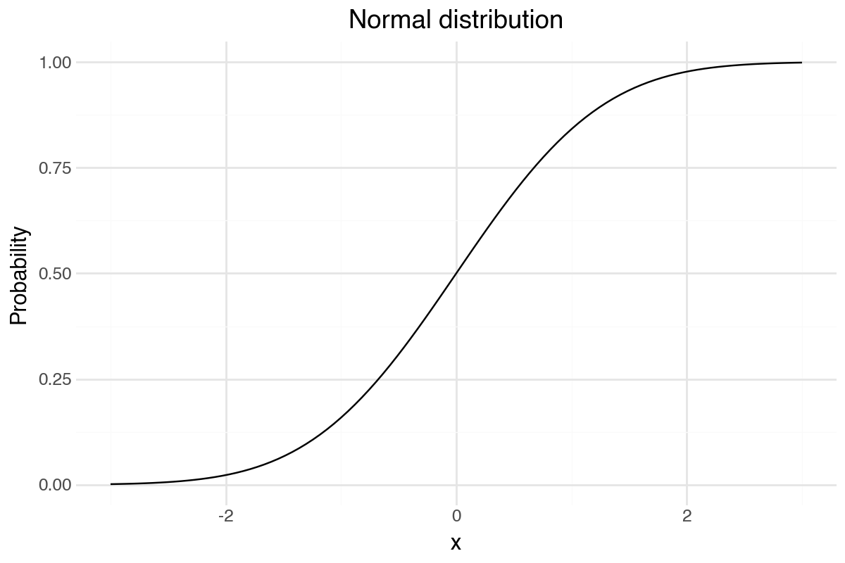
All three languages provide functions for the common distributions — normal, Student-t, chi-square, binomial and others. They provide densities (PDF), distribution functions (CDF), quantile functions (inverse CDF) and random number generation (discussed in Chapter 15).

The first letter of the function name indicates the type: d for density, p for probability, q for quantile and r for random:

dnorm, pnorm, qnorm, rnorm (normal)
dt, pt, qt, rt (Student-t)

cat(sprintf("PDF at 1: %.6f\n", dnorm(1)))
cat(sprintf("CDF at 1.645: %.6f\n", pnorm(1.645)))
cat(sprintf("95th percentile: %.6f\n", qnorm(0.95)))

PDF at 1: 0.241971
CDF at 1.645: 0.950015
95th percentile: 1.644854

Python uses scipy.stats for distribution functions:

print(f"PDF at 1: {norm.pdf(1):.6f}")
print(f"CDF at 1.645: {norm.cdf(1.645):.6f}")
print(f"95th percentile: {norm.ppf(0.95):.6f}")

PDF at 1: 0.241971
CDF at 1.645: 0.950015
95th percentile: 1.644854

Julia uses the Distributions package:

using Printf;
d = Normal(0, 1);
@printf("PDF at 1: %.6f\n", pdf(d, 1))
@printf("CDF at 1.645: %.6f\n", cdf(d, 1.645))
@printf("95th percentile: %.6f\n", quantile(d, 0.95))

PDF at 1: 0.241971
CDF at 1.645: 0.950015
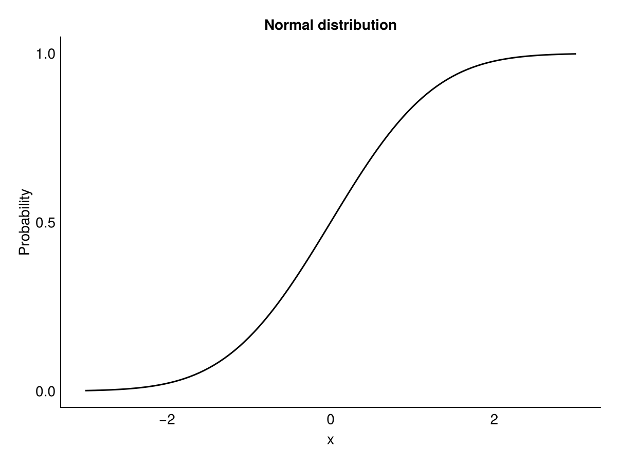
95th percentile: 1.644854

14.3.1 Plotting distributions

df_dist = data.frame(x = seq(-3, 3, length = 100))
df_dist$density = dnorm(df_dist$x)
df_dist$distribution = pnorm(df_dist$x)

ggplot(df_dist, aes(x = x, y = density)) +
  geom_line() +
  labs(title = "Normal density", x = "x", y = "Density") +
  theme_minimal()

ggplot(df_dist, aes(x = x, y = distribution)) +
  geom_line() +
  labs(title = "Normal distribution", x = "x", y = "Probability") +
  theme_minimal()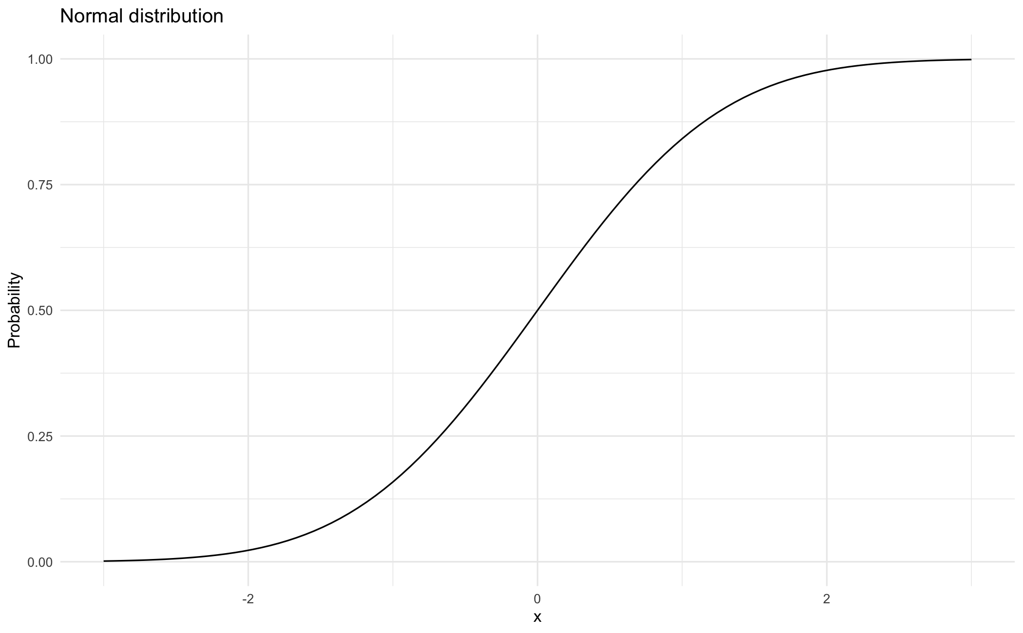

df_dist = pd.DataFrame({'x': np.linspace(-3, 3, 100)})
df_dist['density'] = norm.pdf(df_dist['x'])
df_dist['distribution'] = norm.cdf(df_dist['x'])

p = (ggplot(df_dist, aes(x='x', y='density'))
 + geom_line()
 + labs(title="Normal density", x="x", y="Density")
 + theme_minimal())
p.save("_figs/stats_density_py.png", width=6, height=4, dpi=100, verbose=False)

p = (ggplot(df_dist, aes(x='x', y='distribution'))
 + geom_line()
 + labs(title="Normal distribution", x="x", y="Probability")
 + theme_minimal())
p.save("_figs/stats_cdf_py.png", width=6, height=4, dpi=100, verbose=False)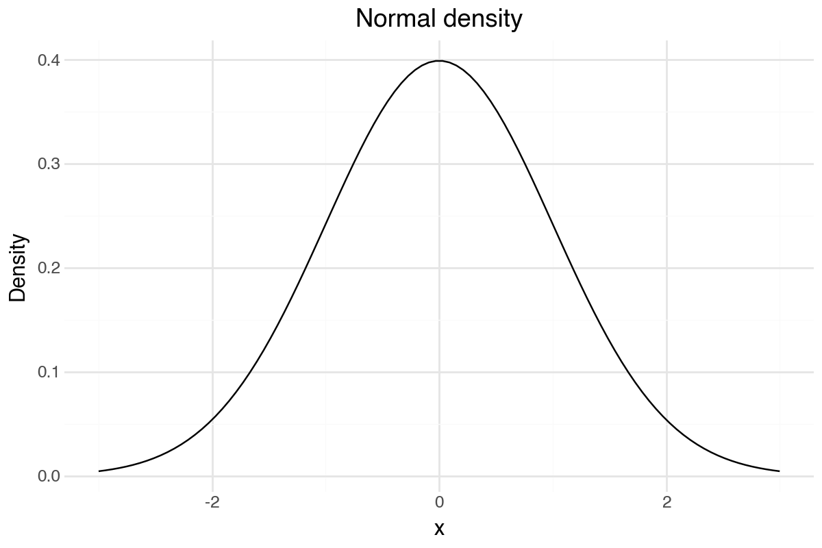

x = range(-3, 3, length=100);
df_dist = DataFrame(x = collect(x), density = pdf.(Normal(), x), distribution = cdf.(Normal(), x));

p = ggplot(df_dist, @aes(x = x, y = density)) +
    geom_line() +
    labs(title = "Normal density", x = "x", y = "Density") +
    theme_minimal();
ggsave("_figs/stats_density_jl.png", p);

p = ggplot(df_dist, @aes(x = x, y = distribution)) +
    geom_line() +
    labs(title = "Normal distribution", x = "x", y = "Probability") +
    theme_minimal();
ggsave("_figs/stats_cdf_jl.png", p);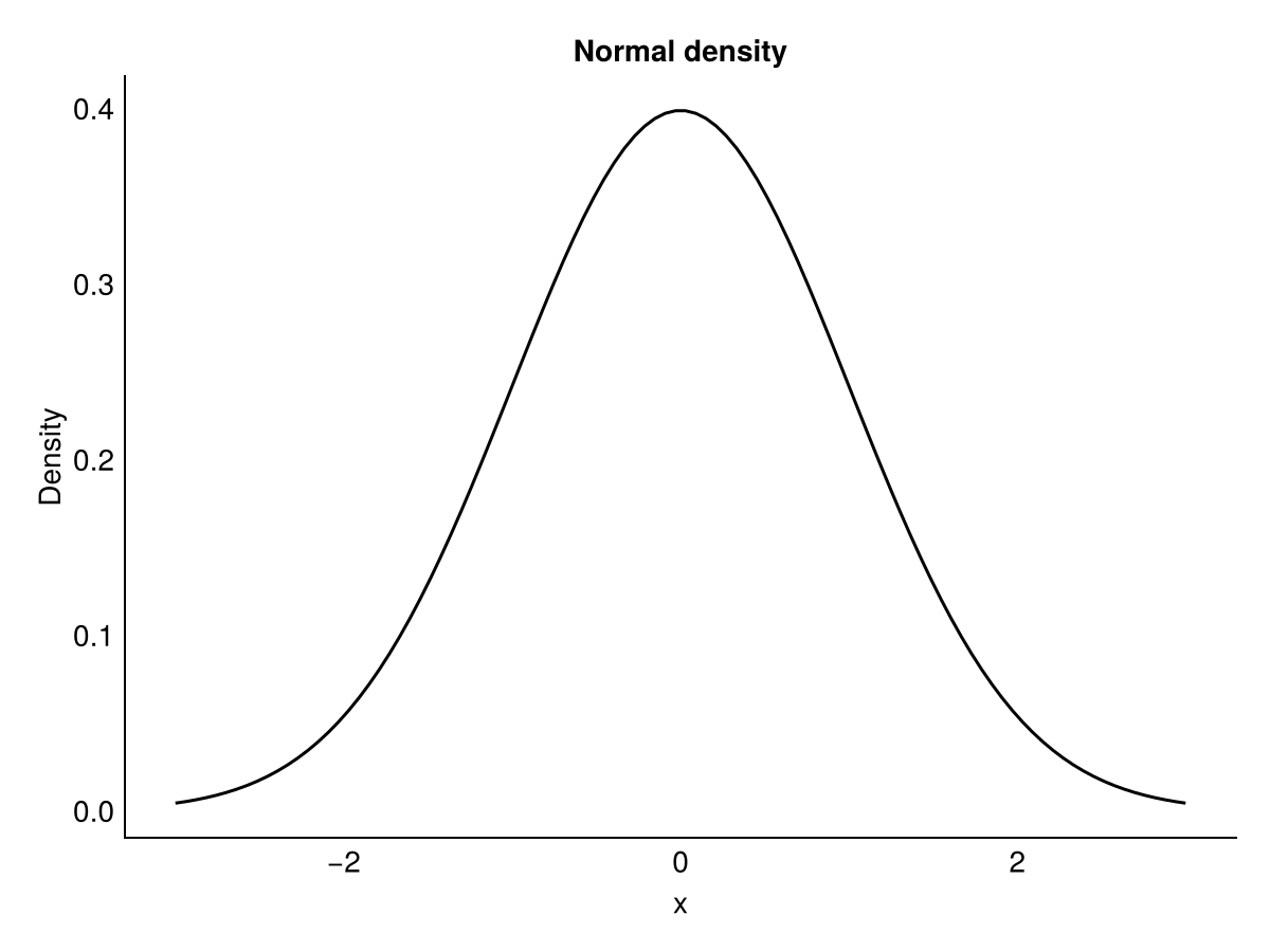

14.3.2 Compare distributions

We start by comparing the normal and Student-t densities. The Student-t is convenient when we need a fat-tailed distribution.

x = seq(-3, 3, length = 500)
df_density = data.frame(
  x = rep(x, 2),
  density = c(dnorm(x), dt(x, df = 2)),
  distribution = rep(c("Normal", "Student-t(2)"), each = length(x))
)

ggplot(df_density, aes(x = x, y = density, colour = distribution)) +
  geom_line(linewidth = 1) +
  scale_colour_manual(values = c("Normal" = "red", "Student-t(2)" = "blue")) +
  labs(title = "Normal vs Student-t densities", x = "Value", y = "Density", colour = NULL) +
  theme_minimal() +
  theme(legend.position = "top")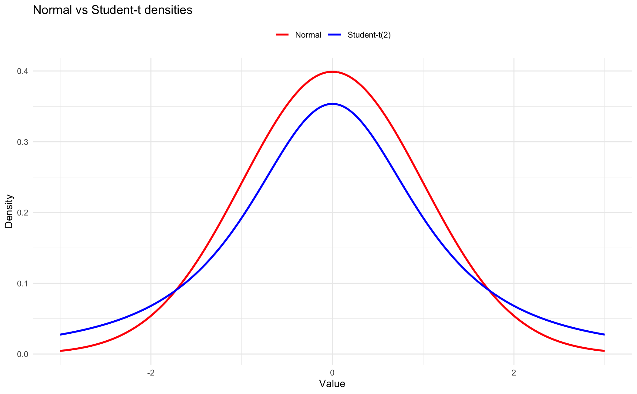

x = np.linspace(-3, 3, 500)
df_density = pd.DataFrame({
    'x': np.tile(x, 2),
    'density': np.concatenate([norm.pdf(x), t.pdf(x, df=2)]),
    'distribution': ['Normal'] * len(x) + ['Student-t(2)'] * len(x)
})

p = (ggplot(df_density, aes(x='x', y='density', color='distribution'))
 + geom_line(size=1)
 + scale_color_manual(values={'Normal': 'red', 'Student-t(2)': 'blue'})
 + labs(title="Normal vs Student-t densities", x="Value", y="Density", color="")
 + theme_minimal()
 + theme(legend_position="top"))
p.save("_figs/stats_compare_py.png", width=6, height=4, dpi=100, verbose=False)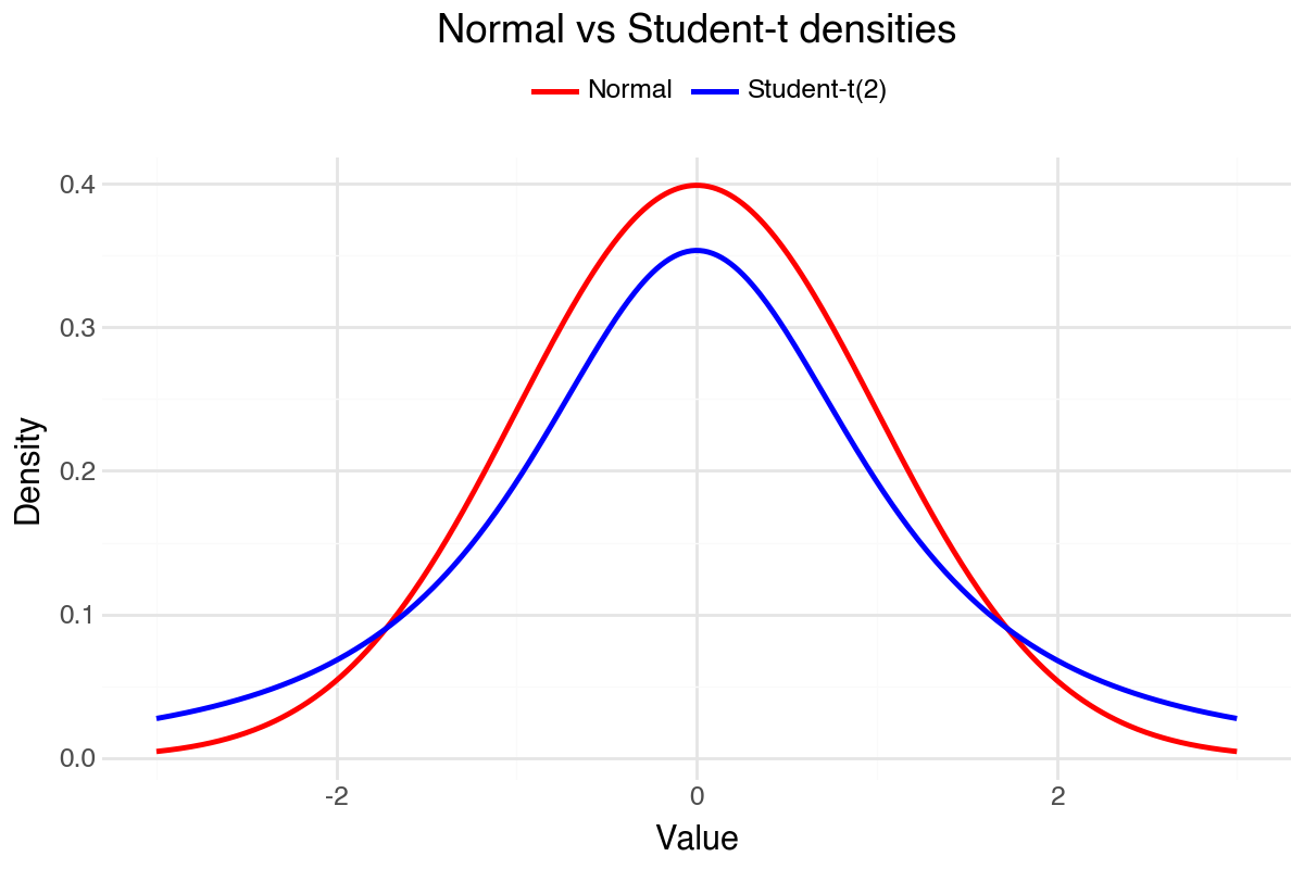

x = range(-3, 3, length=500);
df_density = DataFrame(
    x = vcat(collect(x), collect(x)),
    density = vcat(pdf.(Normal(), x), pdf.(TDist(2), x)),
    distribution = vcat(fill("Normal", length(x)), fill("Student-t(2)", length(x)))
);

p = ggplot(df_density, @aes(x = x, y = density, color = distribution)) +
    geom_line(linewidth = 1) +
    labs(title = "Normal vs Student-t densities", x = "Value", y = "Density") +
    theme_minimal();
ggsave("_figs/stats_compare_jl.png", p);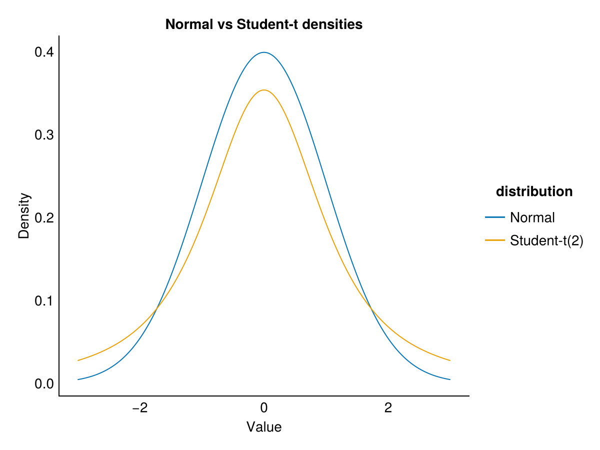

14.4 Testing

We start with formal tests, then turn to the plots.

Three questions matter here. Are returns normally distributed? Do they exhibit serial correlation? How well do they fit theoretical distributions? Each test provides a p-value, the probability under the null hypothesis of a result at least as extreme as the one observed.

14.4.1 Hypothesis tests

14.4.1.1 Jarque-Bera

The Jarque-Bera (JB) test uses the third and fourth central moments of the sample data to check whether its skewness and kurtosis match a normal distribution.

R provides the test in the tseries library:

jb = jarque.bera.test(sp500$y)
cat(sprintf("Jarque-Bera statistic: %.4f\n", jb$statistic))
cat(sprintf("p-value: %.4e\n", jb$p.value))

Jarque-Bera statistic: 43729.8606
p-value: 0.0000e+00

Python provides the test in scipy.stats:

y = sp500['y'].dropna()
stat, pvalue = stats.jarque_bera(y)
print(f"Jarque-Bera statistic: {stat:.4f}")
print(f"p-value: {pvalue:.4e}")

Jarque-Bera statistic: 43729.8606
p-value: 0.0000e+00

Julia provides the test in HypothesisTests:

using Printf;
y = collect(skipmissing(sp500.y));
jb = JarqueBeraTest(y);
@printf("Jarque-Bera statistic: %.4f\n", jb.JB)
@printf("p-value: %.4e\n", pvalue(jb))

Jarque-Bera statistic: 43729.8606
p-value: 0.0000e+00

The p-value is effectively zero. We reject normality.

14.4.1.2 Kolmogorov-Smirnov

The two-sample Kolmogorov–Smirnov test measures the distance between two empirical distributions. We start with two normal samples as a baseline.

We then compare S&P 500 returns against samples from known distributions. The returns are standardised by their own sample mean and standard deviation, while the reference draws are scaled to unit theoretical variance, so the comparison is of shape rather than scale. Because the return side uses estimated parameters, read the resulting D statistic as a descriptive distance between two samples rather than as a formal goodness-of-fit test.

set.seed(42)
x = rnorm(n = length(sp500$y))
z = rnorm(n = length(sp500$y))
result = ks.test(x, z)
cat(sprintf("Two normal samples: D = %.4f, p-value = %.4f\n", result$statistic, result$p.value))

Two normal samples: D = 0.0105, p-value = 0.7061

The p-value is large, as it should be. Both samples are drawn from the same distribution, so there is nothing for the test to detect.

set.seed(42)
ys = (sp500$y - mean(sp500$y)) / sd(sp500$y)
x = rnorm(n = length(ys))
result = ks.test(x, ys)
cat(sprintf("Normal vs S&P 500: D = %.4f, p-value = %.4e\n", result$statistic, result$p.value))
x = rt(df = 3, n = length(ys)) * sqrt(1/3)
result = ks.test(x, ys)
cat(sprintf("t(3) vs S&P 500: D = %.4f, p-value = %.4f\n", result$statistic, result$p.value))

Warning messages:
1: In ks.test.default(x, ys) :
  p-value will be approximate in the presence of ties
2: In ks.test.default(x, ys) :
  p-value will be approximate in the presence of ties

Normal vs S&P 500: D = 0.0917, p-value = 4.2593e-33
t(3) vs S&P 500: D = 0.0228, p-value = 0.0190

np.random.seed(42)
y = sp500['y'].dropna().values
n = len(y)

x = np.random.normal(size=n)
z = np.random.normal(size=n)
stat, pvalue = stats.ks_2samp(x, z)
print(f"Two normal samples: D = {stat:.4f}, p-value = {pvalue:.4f}")

Two normal samples: D = 0.0097, p-value = 0.7910

The p-value is large, as it should be. Both samples are drawn from the same distribution, so there is nothing for the test to detect.

np.random.seed(42)
ys = (y - np.mean(y)) / np.std(y, ddof=1)
x = np.random.normal(size=n)
stat, pvalue = stats.ks_2samp(x, ys)
print(f"Normal vs S&P 500: D = {stat:.4f}, p-value = {pvalue:.4e}")

x = np.random.standard_t(df=3, size=n) * np.sqrt(1/3)
stat, pvalue = stats.ks_2samp(x, ys)
print(f"t(3) vs S&P 500: D = {stat:.4f}, p-value = {pvalue:.4f}")

Normal vs S&P 500: D = 0.0926, p-value = 8.7658e-34
t(3) vs S&P 500: D = 0.0252, p-value = 0.0069

using Random, Printf; Random.seed!(42);
y = collect(skipmissing(sp500.y));
n = length(y);

x = randn(n);
z = randn(n);
result = ApproximateTwoSampleKSTest(x, z);
@printf("Two normal samples: D = %.4f, p-value = %.4f\n", result.δ, pvalue(result))

Two normal samples: D = 0.0169, p-value = 0.1559

The p-value is large, as it should be. Both samples are drawn from the same distribution, so there is nothing for the test to detect.

using Random, Printf, Statistics; Random.seed!(42);
y = collect(skipmissing(sp500.y));
n = length(y);
ys = (y .- mean(y)) ./ std(y);

x = randn(n);
result = ApproximateTwoSampleKSTest(x, ys);
@printf("Normal vs S&P 500: D = %.4f, p-value = %.4e\n", result.δ, pvalue(result))

x = rand(TDist(3), n) .* sqrt(1/3);
result = ApproximateTwoSampleKSTest(x, ys);
@printf("t(3) vs S&P 500: D = %.4f, p-value = %.4f\n", result.δ, pvalue(result))

Normal vs S&P 500: D = 0.0974, p-value = 2.7473e-37
t(3) vs S&P 500: D = 0.0317, p-value = 0.0003

The normal reference sample separates from the data quickly, the largest D statistic of the three comparisons. The t distribution with three degrees of freedom does better, in the sense of a smaller displayed distance, not a formal comparison of p-values. The seed is fixed in each language, so results reproduce on repeated runs within that language, but the numbers differ across languages because each uses a different random number generator.

14.4.1.3 Ljung-Box

The Ljung-Box (LB) test checks whether a series exhibits serial correlation. We test 10 lags throughout, a shorter horizon than the 20-lag summary table in the chapter 1 slides. The conclusion does not depend on that choice.

set.seed(42)
x = rnorm(n = length(sp500$y))
result = Box.test(x, lag = 10, type = "Ljung-Box")
cat(sprintf("Random normal: Q = %.4f, p-value = %.4f\n", result$statistic, result$p.value))
result = Box.test(sp500$y, lag = 10, type = "Ljung-Box")
cat(sprintf("S&P 500 returns: Q = %.4f, p-value = %.4f\n", result$statistic, result$p.value))
result = Box.test(sp500$y^2, lag = 10, type = "Ljung-Box")
cat(sprintf("Squared returns: Q = %.4f, p-value = %.4e\n", result$statistic, result$p.value))

Random normal: Q = 5.0494, p-value = 0.8879
S&P 500 returns: Q = 90.3645, p-value = 0.0000
Squared returns: Q = 7748.6476, p-value = 0.0000e+00

Python provides the Ljung-Box test in statsmodels:

from statsmodels.stats.diagnostic import acorr_ljungbox

np.random.seed(42)
y = sp500['y'].dropna().values
n = len(y)

x = np.random.normal(size=n)
result = acorr_ljungbox(x, lags=[10], return_df=True)
print(f"Random normal: Q = {result['lb_stat'].values[0]:.4f}, p-value = {result['lb_pvalue'].values[0]:.4f}")

result = acorr_ljungbox(y, lags=[10], return_df=True)
print(f"S&P 500 returns: Q = {result['lb_stat'].values[0]:.4f}, p-value = {result['lb_pvalue'].values[0]:.4f}")

result = acorr_ljungbox(y**2, lags=[10], return_df=True)
print(f"Squared returns: Q = {result['lb_stat'].values[0]:.4f}, p-value = {result['lb_pvalue'].values[0]:.4e}")

Random normal: Q = 6.6245, p-value = 0.7604
S&P 500 returns: Q = 90.3645, p-value = 0.0000
Squared returns: Q = 7748.6476, p-value = 0.0000e+00

Julia provides the Ljung-Box test in HypothesisTests:

using Random, Printf; Random.seed!(42);
y = collect(skipmissing(sp500.y));
n = length(y);

x = randn(n);
result = LjungBoxTest(x, 10);
@printf("Random normal: Q = %.4f, p-value = %.4f\n", result.Q, pvalue(result))

result = LjungBoxTest(y, 10);
@printf("S&P 500 returns: Q = %.4f, p-value = %.4f\n", result.Q, pvalue(result))

result = LjungBoxTest(y.^2, 10);
@printf("Squared returns: Q = %.4f, p-value = %.4e\n", result.Q, pvalue(result))

Random normal: Q = 8.3524, p-value = 0.5945
S&P 500 returns: Q = 90.3645, p-value = 0.0000
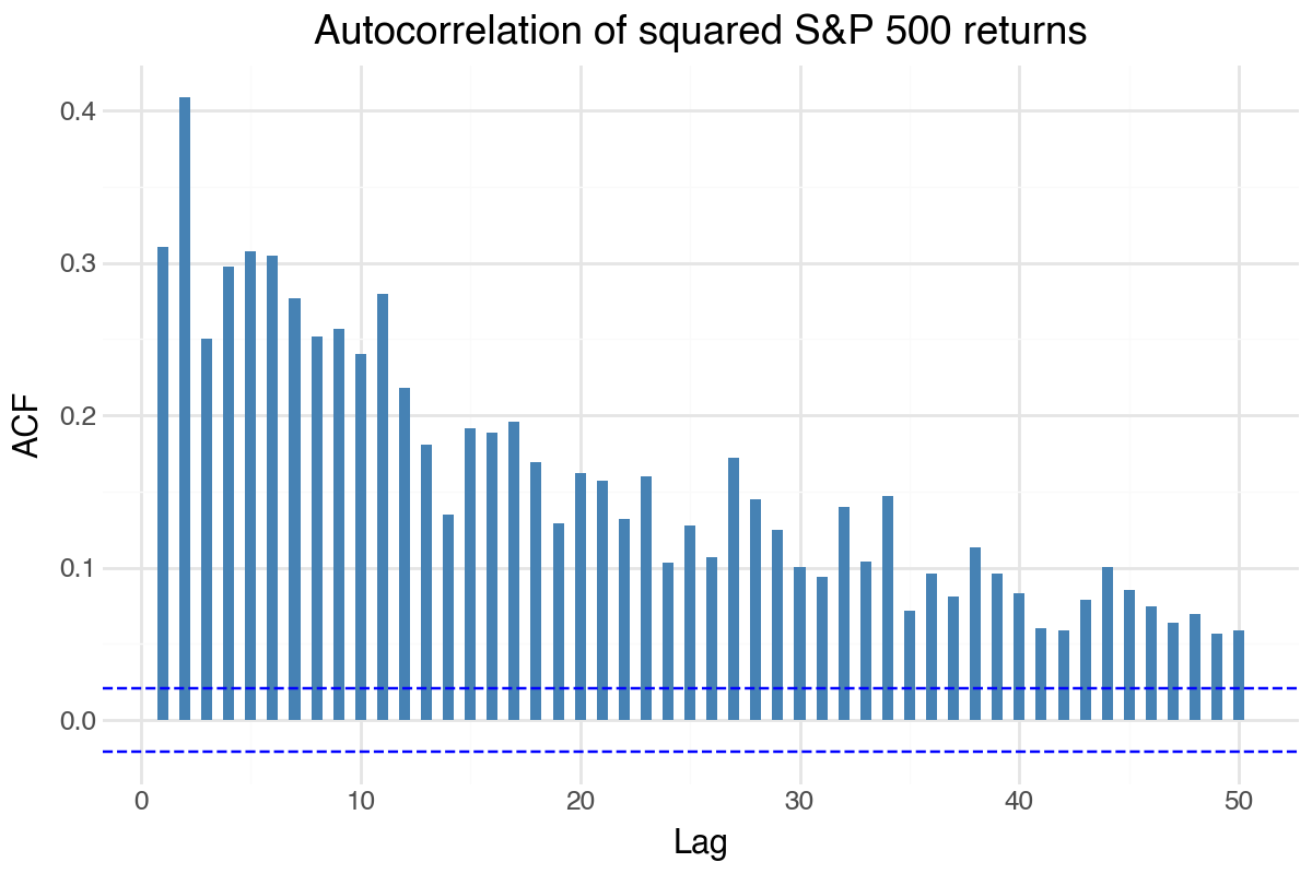
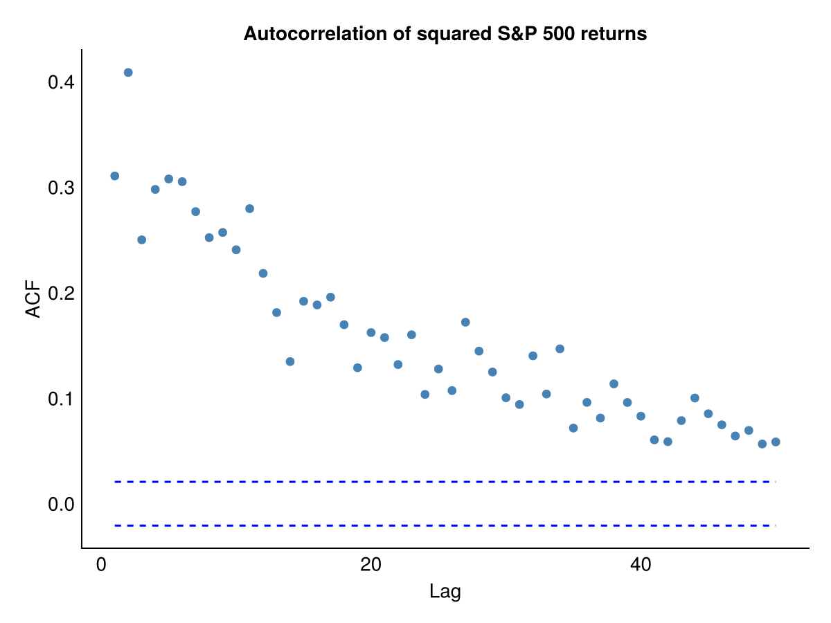
Squared returns: Q = 7748.6476, p-value = 0.0000e+00

The first test on random normal data shows no significant autocorrelation, as expected. The test on S&P 500 returns also rejects the null hypothesis of no autocorrelation, and the rejection for squared returns is far stronger — the signature of volatility clustering, where periods of high volatility tend to be followed by high volatility periods. Volatility clustering is what the GARCH-family models of the later volatility chapters are built to capture.

Read those rejections with care. Both the Ljung–Box \(\chi^2\) calibration and the \(\pm 1.96/\sqrt{\SampleSize}\) bands in the plots below assume the returns are independent under the null. Returns are not. Volatility clustering leaves them dependent even when they are uncorrelated, which inflates the sampling variance of \(\hat{\correlation}_i\) beyond \(1/\SampleSize\). The nominal bands are therefore too narrow and the nominal critical values too low, so both tests reject too readily.

The return autocorrelations here are small in magnitude, and we cannot tell from the nominal calculation alone whether they would survive a calibration that accounts for the dependence.

The squared-return result carries a further condition. The standard asymptotics for \(\hat{\correlation}_i\) applied to \(\CompoundReturns_t^2\) need a finite eighth moment of returns, which is a strong requirement for a fat-tailed series. Treat all of this as a diagnostic that volatility clustering is present, which the plots show unmistakably, rather than as a calibrated test of the conditional mean.

14.4.2 Diagnostic plots

14.4.2.1 Autocorrelation

The autocorrelation function shows the correlation between the series and its own lagged values. The dashed lines are the nominal \(\pm 1.96/\sqrt{\SampleSize}\) reference bands, which is what the plotting packages draw by default. They are the bands for independent observations, so for the reasons above they are too narrow here and a value falling outside them is not by itself evidence of a non-zero autocorrelation. Use them to read the shape of the decay rather than to test individual lags.

The forecast package provides ggAcf() which produces ggplot2-style autocorrelation plots:

ggAcf(sp500$y, lag.max = 50) +
  labs(title = "Autocorrelation of S&P 500 returns") +
  theme_minimal()

ggAcf(sp500$y^2, lag.max = 50) +
  labs(title = "Autocorrelation of squared S&P 500 returns") +
  theme_minimal()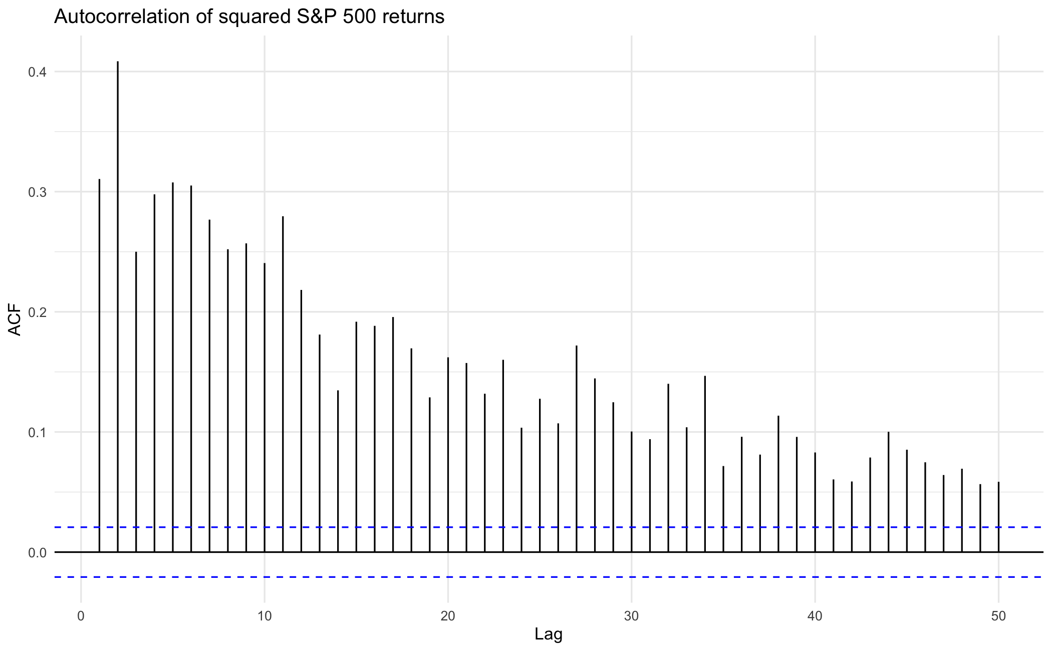

Python uses statsmodels for ACF calculation and plotnine for plotting:

acf_vals = acf(sp500['y'], nlags=50)[1:]
conf_int = 1.96 / np.sqrt(len(sp500['y']))

df_acf = pd.DataFrame({'lag': range(1, len(acf_vals) + 1), 'acf': acf_vals})

p = (ggplot(df_acf, aes(x='lag', y='acf'))
 + geom_bar(stat='identity', fill='steelblue', width=0.5)
 + geom_hline(yintercept=conf_int, linetype='dashed', color='blue')
 + geom_hline(yintercept=-conf_int, linetype='dashed', color='blue')
 + labs(title="Autocorrelation of S&P 500 returns", x="Lag", y="ACF")
 + theme_minimal())
p.save("_figs/stats_acf_py.png", width=6, height=4, dpi=100, verbose=False)

# Squared returns
acf_sq = acf(sp500['y']**2, nlags=50)[1:]
df_acf_sq = pd.DataFrame({'lag': range(1, len(acf_sq) + 1), 'acf': acf_sq})

p = (ggplot(df_acf_sq, aes(x='lag', y='acf'))
 + geom_bar(stat='identity', fill='steelblue', width=0.5)
 + geom_hline(yintercept=conf_int, linetype='dashed', color='blue')
 + geom_hline(yintercept=-conf_int, linetype='dashed', color='blue')
 + labs(title="Autocorrelation of squared S&P 500 returns", x="Lag", y="ACF")
 + theme_minimal())
p.save("_figs/stats_acf_sq_py.png", width=6, height=4, dpi=100, verbose=False)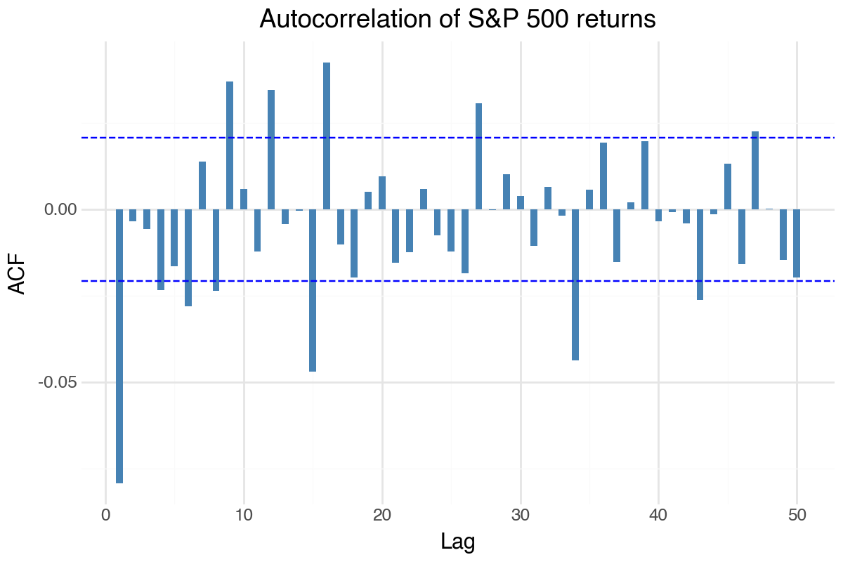

Julia uses StatsBase for ACF calculation:

using StatsBase, DataFrames, TidierPlots
y = collect(skipmissing(sp500.y));

acf_vals = autocor(y, 1:50);
conf_int = 1.96 / sqrt(length(y));

df_acf = DataFrame(lag = 1:50, val = acf_vals);
df_acf.upper .= conf_int;
df_acf.lower .= -conf_int;

p = ggplot(df_acf, @aes(x = lag, y = val)) +
    geom_point(color = "steelblue") +
    geom_line(@aes(x = lag, y = upper), color = "blue", linestyle = :dash) +
    geom_line(@aes(x = lag, y = lower), color = "blue", linestyle = :dash) +
    labs(title = "Autocorrelation of S&P 500 returns", x = "Lag", y = "ACF") +
    theme_minimal();
ggsave("_figs/stats_acf_jl.png", p);

acf_sq = autocor(y .^ 2, 1:50);
df_acf_sq = DataFrame(lag = 1:50, val = acf_sq);
df_acf_sq.upper .= conf_int;
df_acf_sq.lower .= -conf_int;

p = ggplot(df_acf_sq, @aes(x = lag, y = val)) +
    geom_point(color = "steelblue") +
    geom_line(@aes(x = lag, y = upper), color = "blue", linestyle = :dash) +
    geom_line(@aes(x = lag, y = lower), color = "blue", linestyle = :dash) +
    labs(title = "Autocorrelation of squared S&P 500 returns", x = "Lag", y = "ACF") +
    theme_minimal();
ggsave("_figs/stats_acf_sq_jl.png", p);

┌ Warning: Using a `Vector{<:Real}` as a linestyle attribute is deprecated. Wrap it in a `Linestyle`.
└ @ Makie ~/.julia/packages/Makie/Vn16E/src/conversions.jl:1161
┌ Warning: Using a `Vector{<:Real}` as a linestyle attribute is deprecated. Wrap it in a `Linestyle`.
└ @ Makie ~/.julia/packages/Makie/Vn16E/src/conversions.jl:1161
┌ Warning: Using a `Vector{<:Real}` as a linestyle attribute is deprecated. Wrap it in a `Linestyle`.
└ @ Makie ~/.julia/packages/Makie/Vn16E/src/conversions.jl:1161
┌ Warning: Using a `Vector{<:Real}` as a linestyle attribute is deprecated. Wrap it in a `Linestyle`.
└ @ Makie ~/.julia/packages/Makie/Vn16E/src/conversions.jl:1161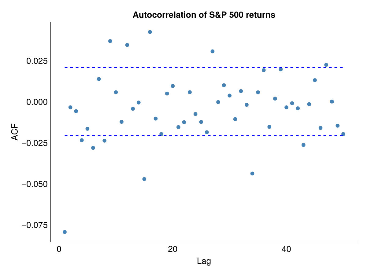

14.4.2.2 QQ-Plots

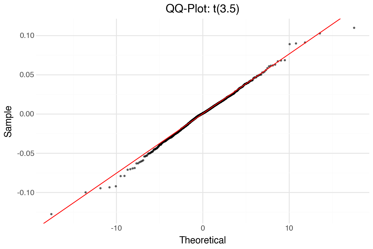
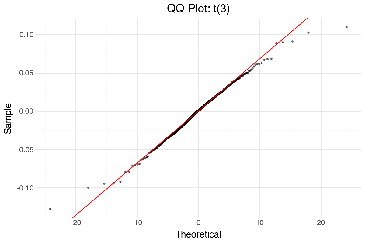
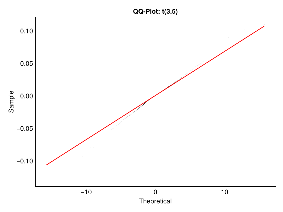
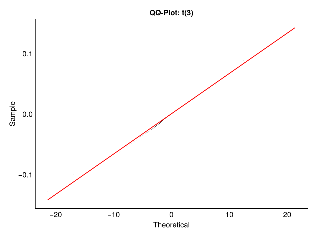
Quantile-quantile (QQ) plots compare the distribution of our data against a theoretical distribution. The line shows the quantiles of the fitted reference distribution. If the data follow that distribution, the points fall on the line. Deviations in the tails reveal departures from the theoretical distribution.

df_qq = data.frame(y = sp500$y)

ggplot(df_qq, aes(sample = y)) +
  stat_qq() +
  stat_qq_line(colour = "red") +
  labs(title = "QQ-Plot: Normal distribution", x = "Theoretical", y = "Sample") +
  theme_minimal()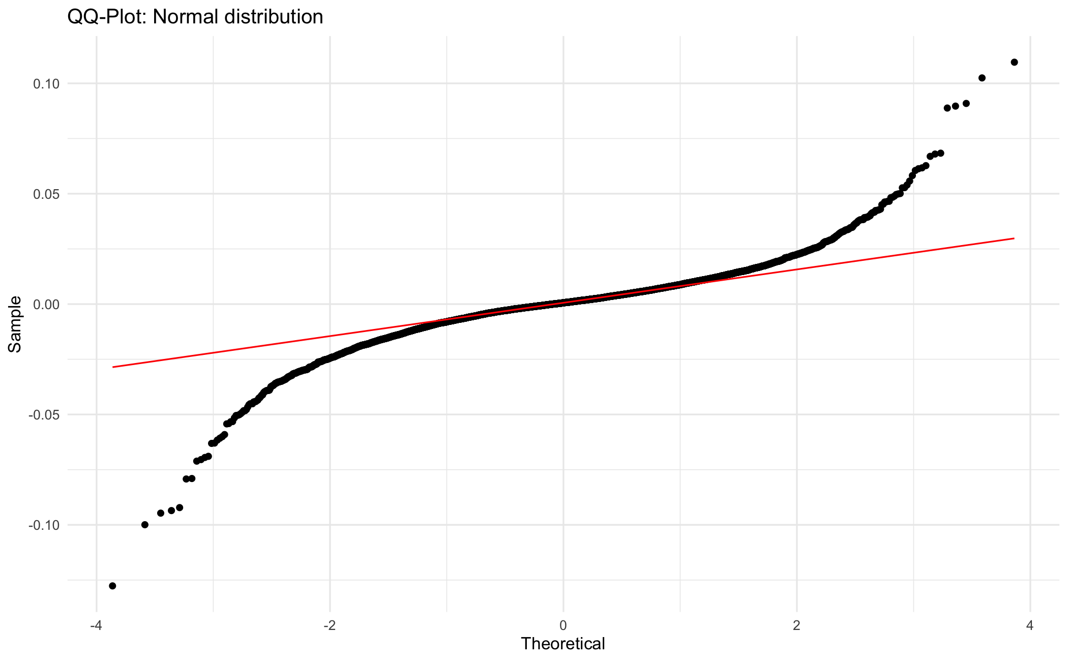

We can also compare against t-distributions with various degrees of freedom. The stat_qq and stat_qq_line functions accept distribution parameters:

df_qq = data.frame(y = sp500$y)

ggplot(df_qq, aes(sample = y)) +
  stat_qq(distribution = qt, dparams = list(df = 4), size = 0.5, alpha = 0.5) +
  stat_qq_line(distribution = qt, dparams = list(df = 4), colour = "red") +
  labs(title = "QQ-Plot: t(4)", x = "Theoretical", y = "Sample") +
  theme_minimal()

ggplot(df_qq, aes(sample = y)) +
  stat_qq(distribution = qt, dparams = list(df = 3.5), size = 0.5, alpha = 0.5) +
  stat_qq_line(distribution = qt, dparams = list(df = 3.5), colour = "red") +
  labs(title = "QQ-Plot: t(3.5)", x = "Theoretical", y = "Sample") +
  theme_minimal()

ggplot(df_qq, aes(sample = y)) +
  stat_qq(distribution = qt, dparams = list(df = 3), size = 0.5, alpha = 0.5) +
  stat_qq_line(distribution = qt, dparams = list(df = 3), colour = "red") +
  labs(title = "QQ-Plot: t(3)", x = "Theoretical", y = "Sample") +
  theme_minimal()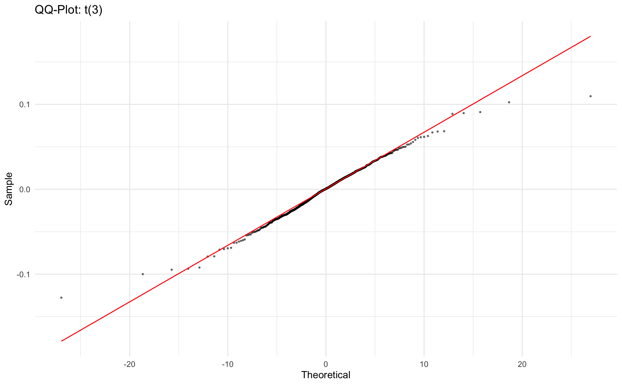

Python uses scipy.stats for QQ plot computation:

from plotnine import geom_abline

y = sp500['y'].dropna().values

# Normal QQ plot
qq = stats.probplot(y, dist="norm")
df_qq = pd.DataFrame({'theoretical': qq[0][0], 'sample': qq[0][1]})
slope, intercept = qq[1][0], qq[1][1]

p = (ggplot(df_qq, aes(x='theoretical', y='sample'))
 + geom_point(size=0.5, alpha=0.5)
 + geom_abline(slope=slope, intercept=intercept, color='red')
 + labs(title="QQ-Plot: Normal distribution", x="Theoretical", y="Sample")
 + theme_minimal())
p.save("_figs/stats_qq_norm_py.png", width=6, height=4, dpi=100, verbose=False)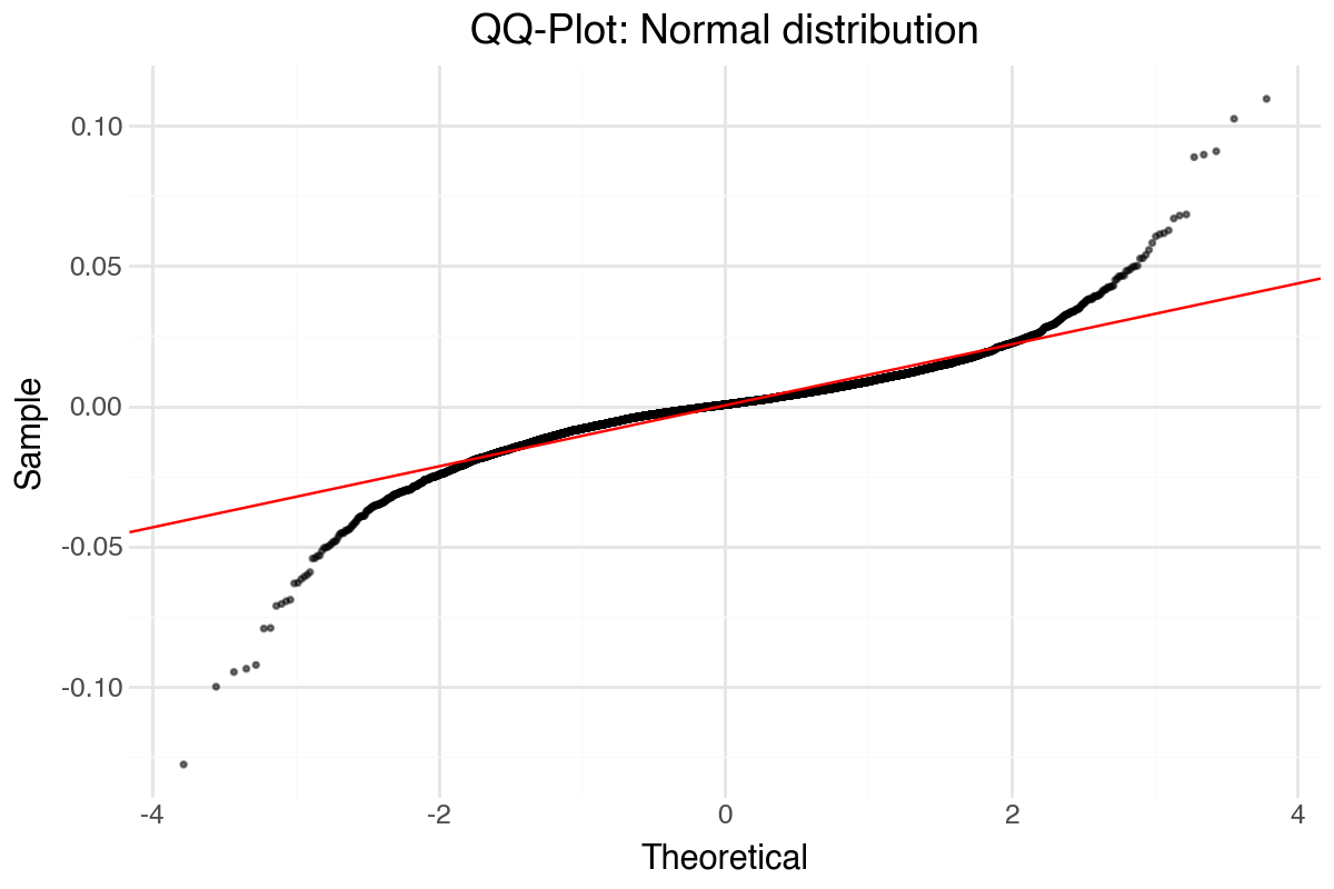

for df_val in [4, 3.5, 3]:
    qq = stats.probplot(y, dist="t", sparams=(df_val,))
    df_qq = pd.DataFrame({'theoretical': qq[0][0], 'sample': qq[0][1]})
    slope, intercept = qq[1][0], qq[1][1]

    p = (ggplot(df_qq, aes(x='theoretical', y='sample'))
     + geom_point(size=0.5, alpha=0.5)
     + geom_abline(slope=slope, intercept=intercept, color='red')
     + labs(title=f"QQ-Plot: t({df_val})", x="Theoretical", y="Sample")
     + theme_minimal())
    p.save(f"_figs/stats_qq_t{df_val}_py.png", width=6, height=4, dpi=100, verbose=False)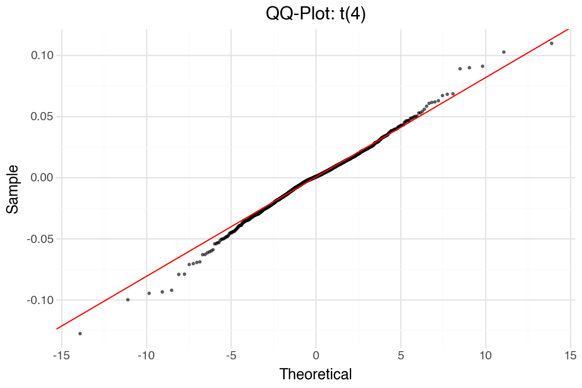

Julia uses Distributions for theoretical quantiles:

y = sort(collect(skipmissing(sp500.y)));
n = length(y);
theoretical = quantile.(Normal(), (1:n) ./ (n + 1));

df_qq = DataFrame(theoretical = theoretical, sample = y);

# QQ line through 1st and 3rd quartiles
q1_t = quantile(Normal(), 0.25); q3_t = quantile(Normal(), 0.75);
q1_s = quantile(y, 0.25); q3_s = quantile(y, 0.75);
slope = (q3_s - q1_s) / (q3_t - q1_t);
intercept = q1_s - slope * q1_t;
df_qq.fit = intercept .+ slope .* df_qq.theoretical;

p = ggplot(df_qq, @aes(x = theoretical, y = sample)) +
    geom_point(size = 0.5, alpha = 0.5) +
    geom_line(@aes(x = theoretical, y = fit), color = "red") +
    labs(title = "QQ-Plot: Normal distribution", x = "Theoretical", y = "Sample") +
    theme_minimal();
ggsave("_figs/stats_qq_norm_jl.png", p);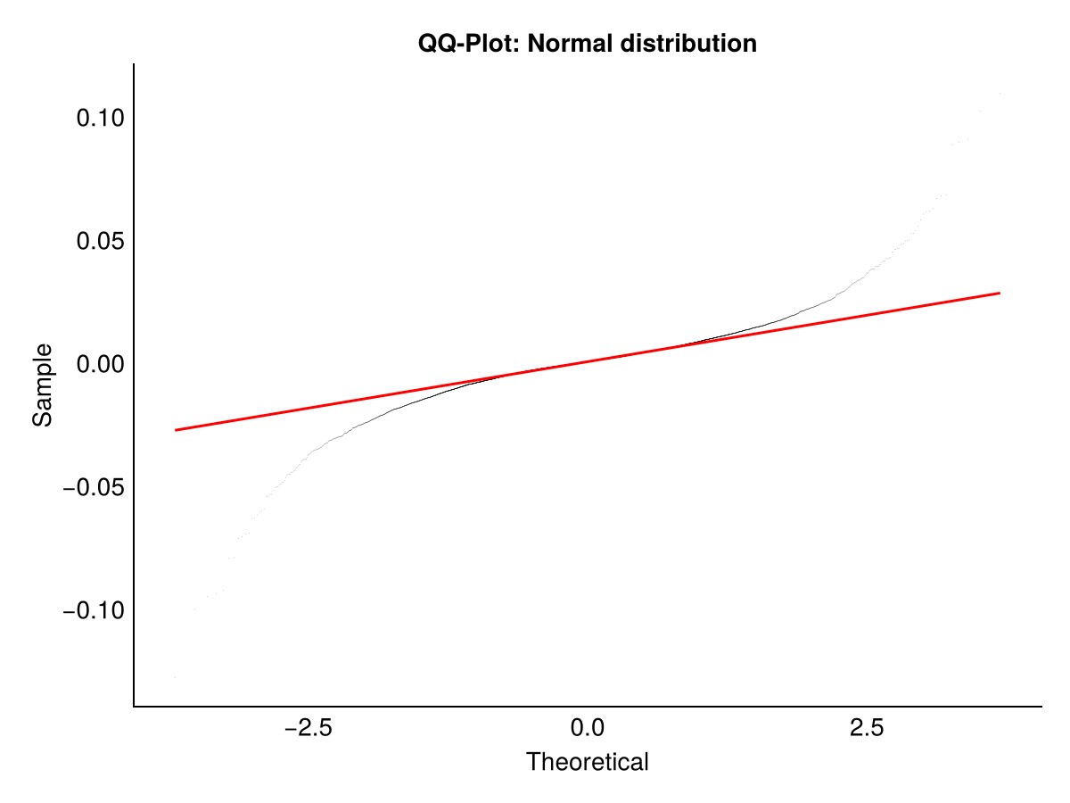

y = sort(collect(skipmissing(sp500.y)));
n = length(y);

for df_val in [4, 3.5, 3]
    df_label = isinteger(df_val) ? string(Int(df_val)) : string(df_val);
    d = TDist(df_val);
    theoretical = quantile.(d, (1:n) ./ (n + 1));
    df_qq = DataFrame(theoretical = theoretical, sample = y);

    q1_t = quantile(d, 0.25); q3_t = quantile(d, 0.75);
    q1_s = quantile(y, 0.25); q3_s = quantile(y, 0.75);
    slope = (q3_s - q1_s) / (q3_t - q1_t);
    intercept = q1_s - slope * q1_t;
    df_qq.fit = intercept .+ slope .* df_qq.theoretical;

    p = ggplot(df_qq, @aes(x = theoretical, y = sample)) +
        geom_point(size = 0.5, alpha = 0.5) +
        geom_line(@aes(x = theoretical, y = fit), color = "red") +
        labs(title = "QQ-Plot: t($df_label)", x = "Theoretical", y = "Sample") +
        theme_minimal();
    ggsave("_figs/stats_qq_t$(df_label)_jl.png", p);
end;

┌ Warning: Assignment to `d` in soft scope is ambiguous because a global variable by the same name exists: `d` will be treated as a new local. Disambiguate by using `local d` to suppress this warning or `global d` to assign to the existing global variable.
└ @ ~/github/notebook/_prebake/Programming/Stats/prebake.jl:239
┌ Warning: Assignment to `theoretical` in soft scope is ambiguous because a global variable by the same name exists: `theoretical` will be treated as a new local. Disambiguate by using `local theoretical` to suppress this warning or `global theoretical` to assign to the existing global variable.
└ @ ~/github/notebook/_prebake/Programming/Stats/prebake.jl:240
┌ Warning: Assignment to `df_qq` in soft scope is ambiguous because a global variable by the same name exists: `df_qq` will be treated as a new local. Disambiguate by using `local df_qq` to suppress this warning or `global df_qq` to assign to the existing global variable.
└ @ ~/github/notebook/_prebake/Programming/Stats/prebake.jl:241
┌ Warning: Assignment to `q1_t` in soft scope is ambiguous because a global variable by the same name exists: `q1_t` will be treated as a new local. Disambiguate by using `local q1_t` to suppress this warning or `global q1_t` to assign to the existing global variable.
└ @ ~/github/notebook/_prebake/Programming/Stats/prebake.jl:243
┌ Warning: Assignment to `q3_t` in soft scope is ambiguous because a global variable by the same name exists: `q3_t` will be treated as a new local. Disambiguate by using `local q3_t` to suppress this warning or `global q3_t` to assign to the existing global variable.
└ @ ~/github/notebook/_prebake/Programming/Stats/prebake.jl:243
┌ Warning: Assignment to `q1_s` in soft scope is ambiguous because a global variable by the same name exists: `q1_s` will be treated as a new local. Disambiguate by using `local q1_s` to suppress this warning or `global q1_s` to assign to the existing global variable.
└ @ ~/github/notebook/_prebake/Programming/Stats/prebake.jl:244
┌ Warning: Assignment to `q3_s` in soft scope is ambiguous because a global variable by the same name exists: `q3_s` will be treated as a new local. Disambiguate by using `local q3_s` to suppress this warning or `global q3_s` to assign to the existing global variable.
└ @ ~/github/notebook/_prebake/Programming/Stats/prebake.jl:244
┌ Warning: Assignment to `slope` in soft scope is ambiguous because a global variable by the same name exists: `slope` will be treated as a new local. Disambiguate by using `local slope` to suppress this warning or `global slope` to assign to the existing global variable.
└ @ ~/github/notebook/_prebake/Programming/Stats/prebake.jl:245
┌ Warning: Assignment to `intercept` in soft scope is ambiguous because a global variable by the same name exists: `intercept` will be treated as a new local. Disambiguate by using `local intercept` to suppress this warning or `global intercept` to assign to the existing global variable.
└ @ ~/github/notebook/_prebake/Programming/Stats/prebake.jl:246
┌ Warning: Assignment to `p` in soft scope is ambiguous because a global variable by the same name exists: `p` will be treated as a new local. Disambiguate by using `local p` to suppress this warning or `global p` to assign to the existing global variable.
└ @ ~/github/notebook/_prebake/Programming/Stats/prebake.jl:249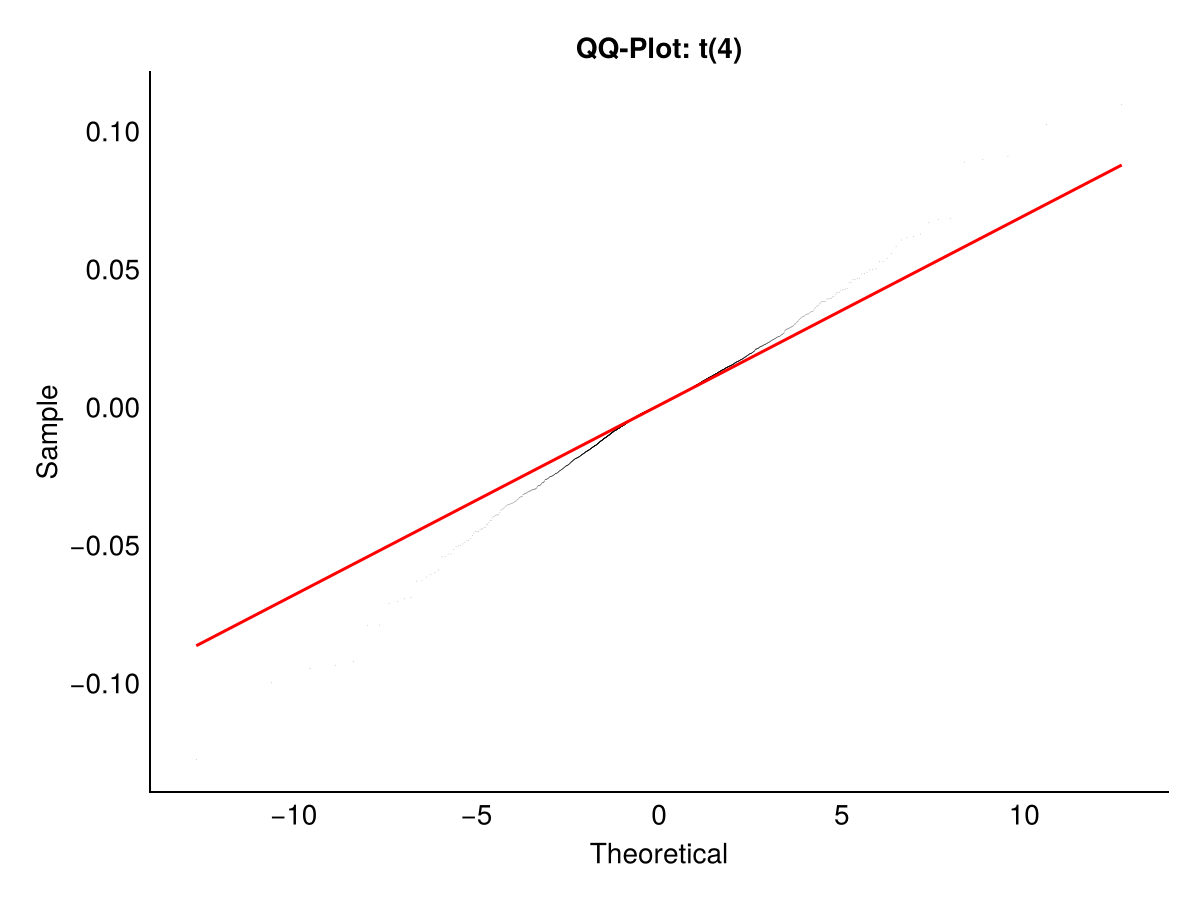

14.5 Return distribution analysis

Numbers alone do not settle the question. A plot shows immediately what a table can hide.

The mean-variance framework assumes returns are normally distributed. In reality, stock returns are heavy-tailed and skewed. See Section 12.6 for basic histogram syntax. Here we compare the empirical distribution to the normal.

14.5.1 Histogram/density

ggplot(sp500, aes(x = y)) +
  geom_histogram(aes(y = after_stat(density)), bins = 30,
                 fill = "deepskyblue3", colour = "white") +
  stat_function(fun = dnorm, args = list(mean = mean(sp500$y), sd = sd(sp500$y)),
                colour = "red", linewidth = 1, linetype = "dashed") +
  labs(title = "S&P 500 histogram with normal overlay", x = "Return", y = "Density") +
  theme_minimal()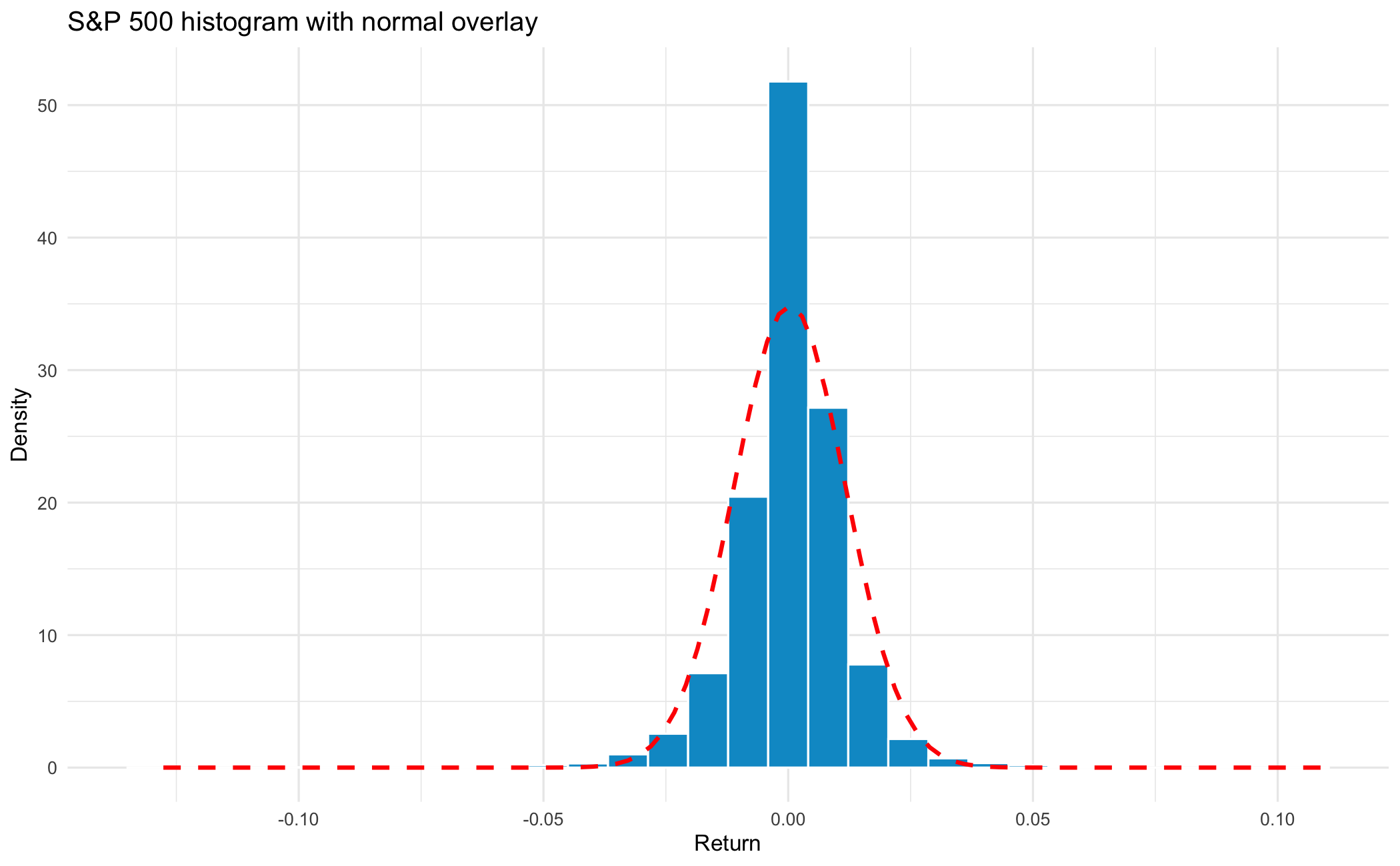

from plotnine import after_stat

x_range = np.linspace(sp500['y'].min(), sp500['y'].max(), 100)
normal_pdf = norm.pdf(x_range, sp500['y'].mean(), sp500['y'].std())
df_norm = pd.DataFrame({'x': x_range, 'pdf': normal_pdf})

p = (ggplot(sp500, aes(x='y'))
 + geom_histogram(aes(y=after_stat("density")), bins=30, fill='deepskyblue', color='white')
 + geom_line(data=df_norm, mapping=aes(x='x', y='pdf'), color='red', size=1, linetype='dashed')
 + labs(title="S&P 500 histogram with normal overlay", x="Return", y="Density")
 + theme_minimal())
p.save("_figs/stats_hist_py.png", width=6, height=4, dpi=100, verbose=False)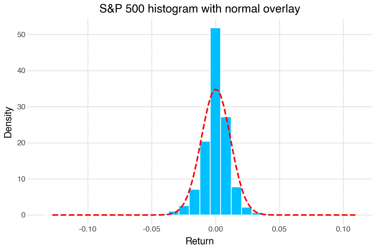

y = collect(skipmissing(sp500.y));
df_hist = DataFrame(y = y);

# Compute histogram bins for density normalisation
h = fit(Histogram, y, nbins=30);
edges = collect(h.edges[1]);
bw = edges[2] - edges[1];
counts = h.weights;
density_vals = counts ./ (sum(counts) * bw);
mids = (edges[1:end-1] .+ edges[2:end]) ./ 2;
df_bars = DataFrame(x = mids, density = density_vals);

# Normal overlay
x_range = range(minimum(y), maximum(y), length=100);
df_norm = DataFrame(x = collect(x_range), pdf = pdf.(Normal(mean(y), std(y)), x_range));

p = ggplot(df_bars, @aes(x = x, y = density)) +
    geom_col(color = "deepskyblue", width = bw) +
    geom_line(df_norm, @aes(x = x, y = pdf), color = "red", linewidth = 1, linestyle = :dash) +
    labs(title = "S&P 500 histogram with normal overlay", x = "Return", y = "Density") +
    theme_minimal();
ggsave("_figs/stats_hist_jl.png", p);

┌ Warning: Using a `Vector{<:Real}` as a linestyle attribute is deprecated. Wrap it in a `Linestyle`.
└ @ Makie ~/.julia/packages/Makie/Vn16E/src/conversions.jl:1161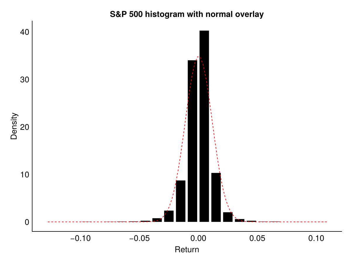

From the plots, we see that although the empirical distribution has a bell shape, the returns have fat tails and are skewed. Returns near the mean occur more often than the normal distribution predicts, so S&P 500 returns do not look normal.

14.5.2 Box plot

ggplot(sp500, aes(y = y)) +
  geom_boxplot(fill = "deepskyblue3", width = 0.5) +
  labs(title = "Box Plot - S&P 500", y = "Return") +
  theme_minimal() +
  theme(axis.text.x = element_blank(), axis.ticks.x = element_blank())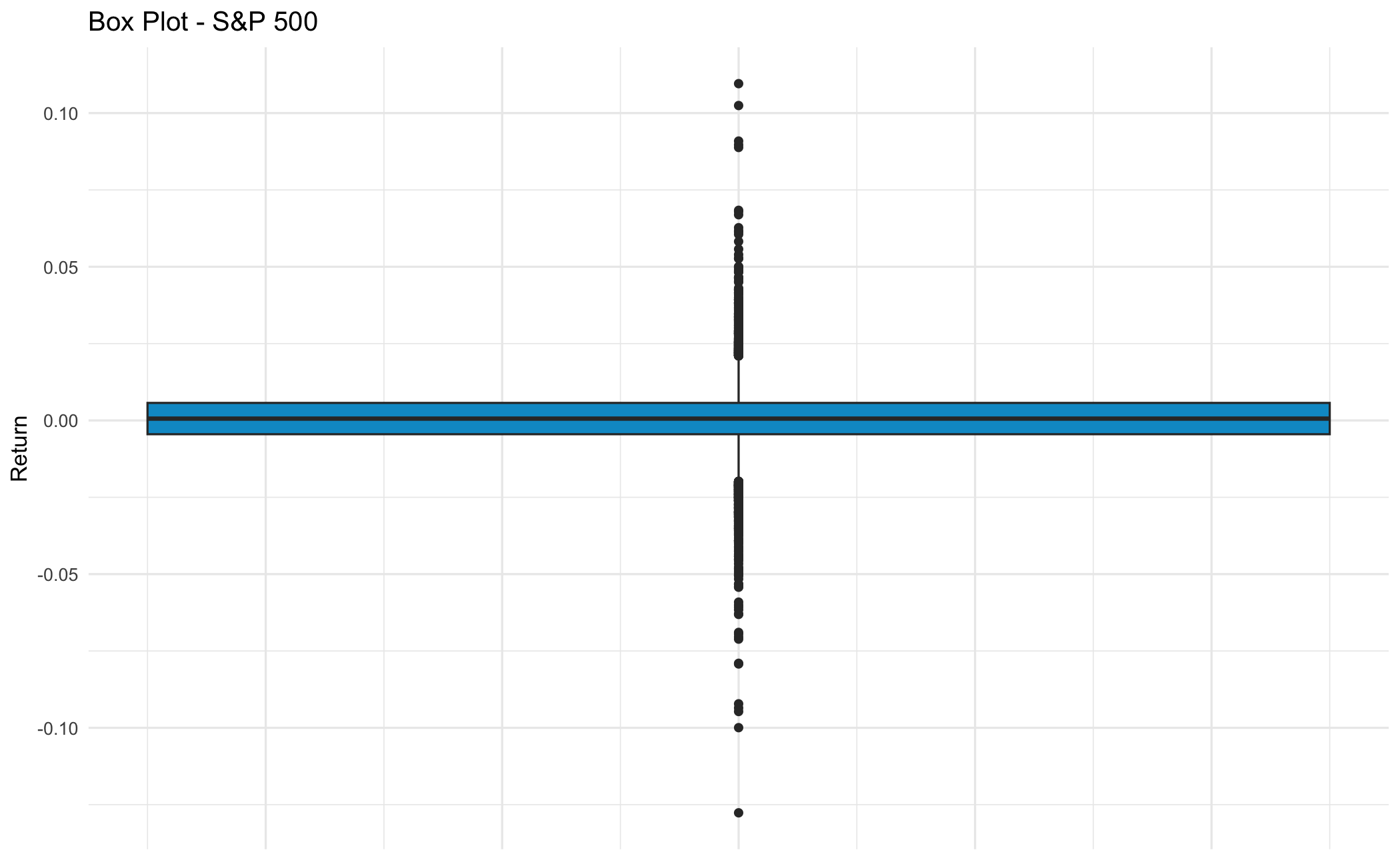

p = (ggplot(sp500, aes(x='""', y='y'))
 + geom_boxplot(fill='deepskyblue')
 + labs(title="Box Plot - S&P 500", y="Return", x="")
 + theme_minimal())
p.save("_figs/stats_box_py.png", width=4, height=4, dpi=100, verbose=False)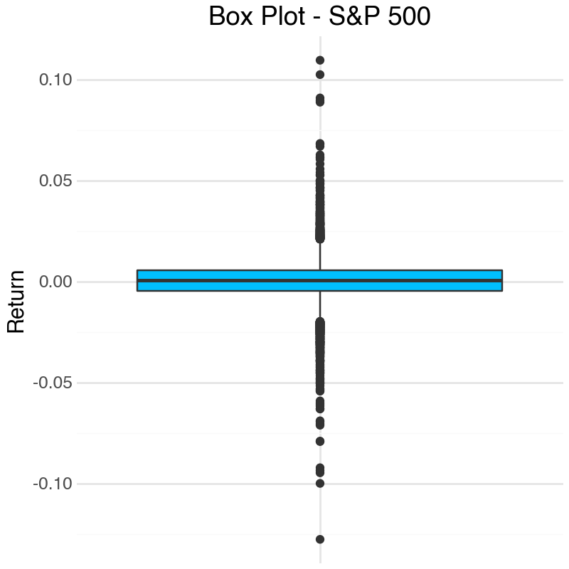

df_box = DataFrame(y = collect(skipmissing(sp500.y)));

p = ggplot(df_box, @aes(x = "", y = y)) +
    geom_boxplot(fill = "deepskyblue") +
    labs(title = "Box Plot - S&P 500", y = "Return", x = "") +
    theme_minimal();
ggsave("_figs/stats_box_jl.png", p, width = 400, height = 400);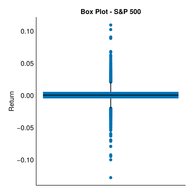

The box plot shows many outliers in S&P 500 returns. This indicates that unusually high or low returns are not rare.

14.5.3 Empirical distribution

The stat_ecdf() function generates the empirical cumulative distribution:

ggplot(sp500, aes(x = y)) +
  stat_ecdf(colour = "blue") +
  stat_function(fun = pnorm, args = list(mean = mean(sp500$y), sd = sd(sp500$y)),
                colour = "red") +
  labs(title = "S&P 500 empirical distribution and the normal",
       x = "Returns", y = "Probability") +
  theme_minimal()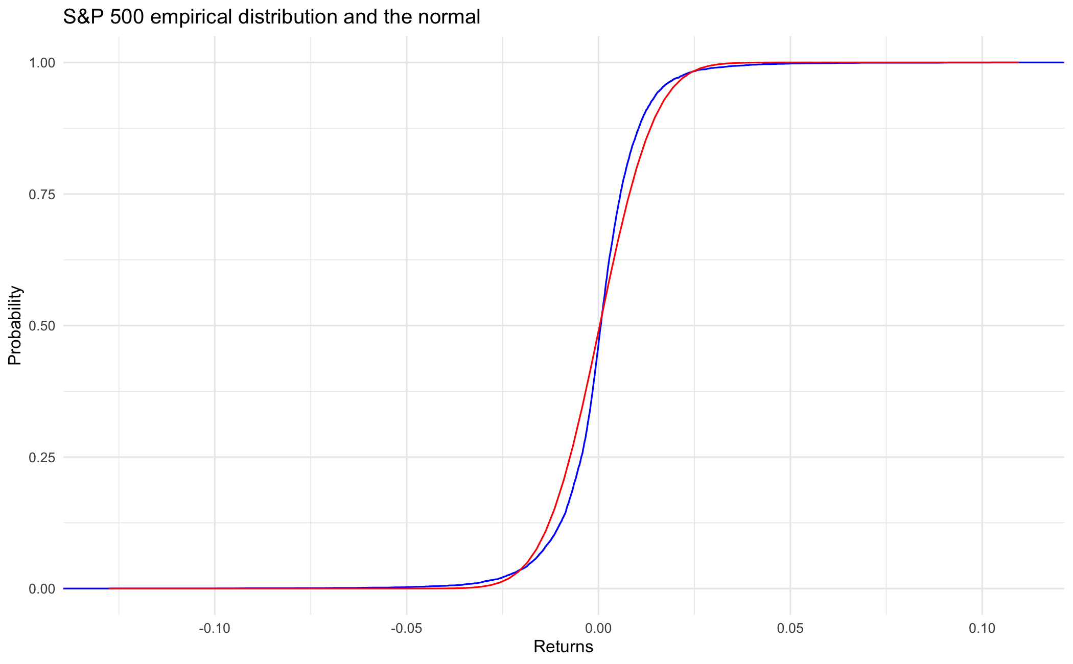

x_sorted = np.sort(sp500['y'])
ecdf = np.arange(1, len(x_sorted) + 1) / len(x_sorted)
df_ecdf = pd.DataFrame({'x': x_sorted, 'ecdf': ecdf})

x_norm = np.linspace(sp500['y'].min(), sp500['y'].max(), 100)
cdf_norm = norm.cdf(x_norm, sp500['y'].mean(), sp500['y'].std())
df_norm = pd.DataFrame({'x': x_norm, 'cdf': cdf_norm})

p = (ggplot()
 + geom_step(data=df_ecdf, mapping=aes(x='x', y='ecdf'), color='blue')
 + geom_line(data=df_norm, mapping=aes(x='x', y='cdf'), color='red')
 + labs(title="S&P 500 empirical distribution and the normal", x="Returns", y="Probability")
 + theme_minimal())
p.save("_figs/stats_ecdf_py.png", width=6, height=4, dpi=100, verbose=False)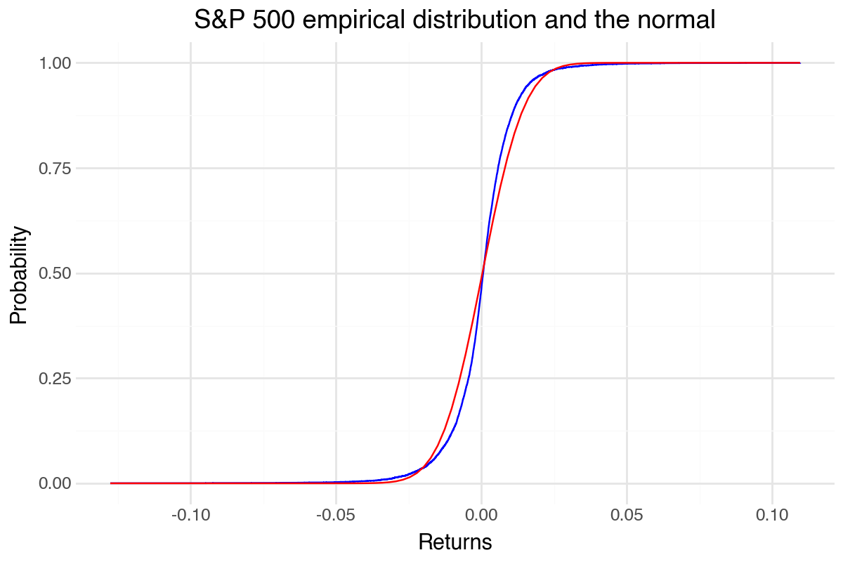

using Statistics, Distributions, DataFrames, TidierPlots
x_sorted = sort(sp500.y);
ecdf_vals = collect(1:length(x_sorted)) ./ length(x_sorted);
df_ecdf = DataFrame(x = x_sorted, prob = ecdf_vals);

xgrid = range(minimum(sp500.y), maximum(sp500.y), length = 200);
cdf_norm = cdf.(Normal(mean(sp500.y), std(sp500.y)), xgrid);
df_norm = DataFrame(x = collect(xgrid), prob = cdf_norm);

p = ggplot(df_ecdf, @aes(x = x, y = prob)) +
    geom_step(color = "blue") +
    geom_line(@aes(x = x, y = prob), data = df_norm, color = "red") +
    labs(title = "S&P 500 empirical distribution and the normal", x = "Returns", y = "Probability") +
    theme_minimal();
ggsave("_figs/stats_ecdf_jl.png", p);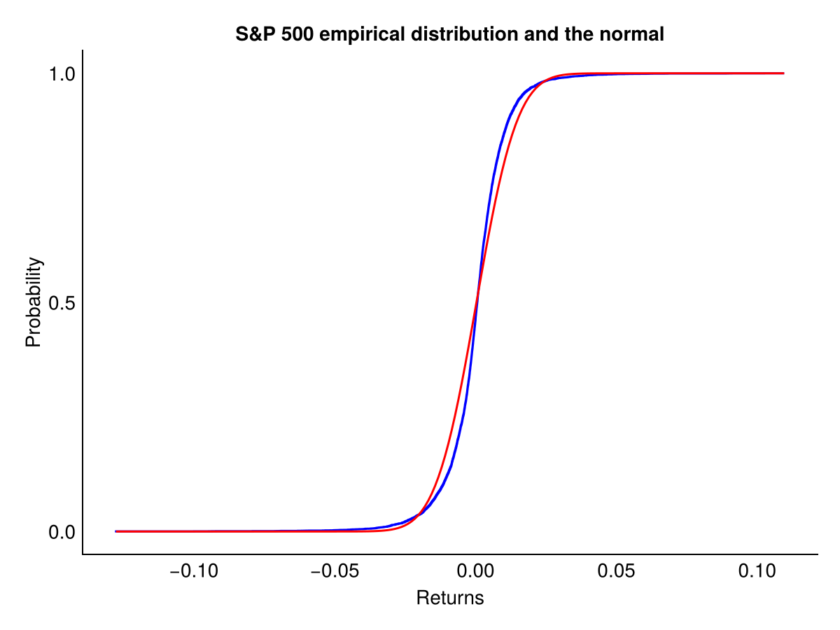

14.5.4 Comparing stock distributions

df_stocks = data.frame(
  returns = c(Return$AAPL, Return$JPM),
  stock = rep(c("AAPL", "JPM"), each = nrow(Return))
)

ggplot(df_stocks, aes(x = returns, colour = stock)) +
  stat_ecdf() +
  scale_colour_manual(values = c("AAPL" = "blue", "JPM" = "red")) +
  labs(title = "Apple and JPMorgan", x = "Returns", y = "Probability", colour = NULL) +
  theme_minimal() +
  theme(legend.position = "top")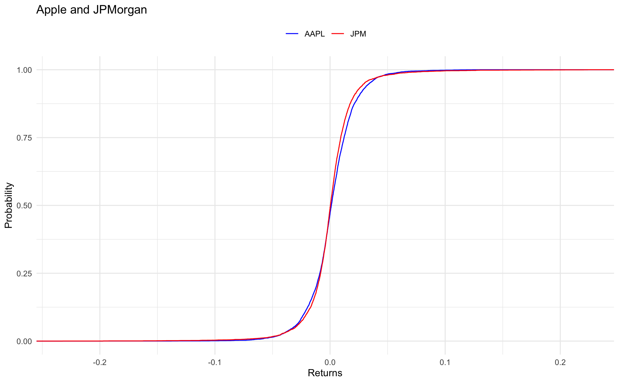

df_stocks = pd.DataFrame({
    'returns': np.concatenate([Return['AAPL'].values, Return['JPM'].values]),
    'stock': ['AAPL'] * len(Return) + ['JPM'] * len(Return)
})

p = (ggplot(df_stocks, aes(x='returns', color='stock'))
 + stat_ecdf()
 + scale_color_manual(values={'AAPL': 'blue', 'JPM': 'red'})
 + labs(title="Apple and JPMorgan", x="Returns", y="Probability", color="")
 + theme_minimal()
 + theme(legend_position="top"))
p.save("_figs/stats_ecdf_stocks_py.png", width=6, height=4, dpi=100, verbose=False)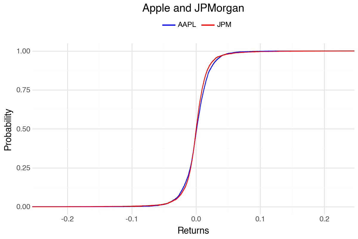

# Sort and compute ECDF for each stock
aapl_sorted = sort(Return.AAPL);
jpm_sorted = sort(Return.JPM);
n = length(aapl_sorted);
df_ecdf = DataFrame(
    x = vcat(aapl_sorted, jpm_sorted),
    ecdf = vcat(collect(1:n) ./ n, collect(1:n) ./ n),
    stock = vcat(fill("AAPL", n), fill("JPM", n))
);

p = ggplot(df_ecdf, @aes(x = x, y = ecdf, color = stock)) +
    geom_step() +
    labs(title = "Apple and JPMorgan", x = "Returns", y = "Probability") +
    theme_minimal();
ggsave("_figs/stats_ecdf_stocks_jl.png", p);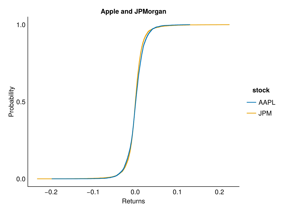

By looking at the tails, we can see which of the two stocks delivers more large returns. JPM has the fatter upper tail, consistent with its higher excess kurtosis reported earlier. Zooming into the upper tail makes the difference visible. The comparison would look the same in Python or Julia, so we show it once, in R:

ggplot(df_stocks, aes(x = returns, colour = stock)) +
  stat_ecdf() +
  scale_colour_manual(values = c("AAPL" = "blue", "JPM" = "red")) +
  coord_cartesian(xlim = c(0.02, 0.1), ylim = c(0.83, 1)) +
  labs(title = "Apple and JPMorgan - upper tail", x = "Returns", y = "Probability", colour = NULL) +
  theme_minimal() +
  theme(legend.position = "bottom")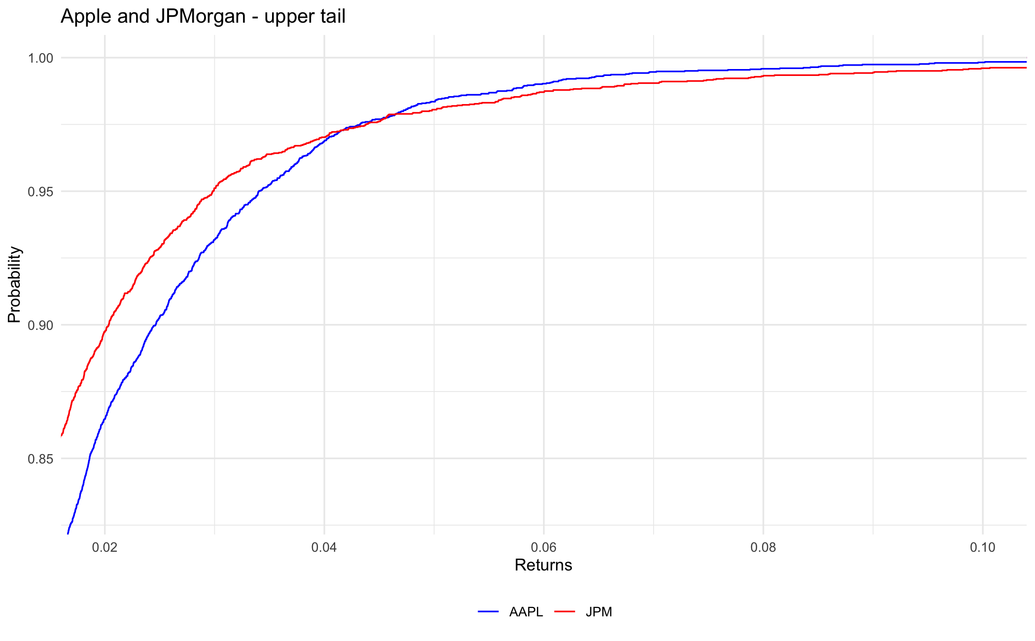

14.6 What the data show

For S&P 500 returns, the Jarque-Bera test rejects normality, and the Ljung-Box test rejects independence far more strongly for squared returns than for the returns themselves, the volatility-clustering signature seen in the plots above. Returns cluster more tightly around the mean than the normal distribution predicts, with fatter tails and skewness that switches sign across the six stocks compared earlier. JPM and AAPL differ too, in the shape of their upper tails.

14.7 Exercise

Load data/stocks.csv via ProcessRawData() in your language of choice, then compute descriptive statistics for all stocks in the Return data frame. Summarise and present the results in a new data frame. It should include mean, standard deviation, skewness, kurtosis and the p-value of the Jarque-Bera test. Keep five decimal places.